Recently, I came across the NAR breakthrough article titled 'Crystal Structure of the Class V GTP-Binding RNA Aptamer Bound to Its Ligand: GTP Recognition by a Topologically Complex Intermolecular G-Quadruplex' by Stafflinger et al. (2025). I read the paper carefully several times and really enjoyed both the content and the writing style. This work offers new insights into the structural complexities and ligand recognition capabilities of RNA. The 1.6-Å high-resolution X-ray crystal structure (PDB id: 9hrf) of the aptamer–GTP complex explains why the class V GTP aptamer has a particularly high affinity and specificity for GTP: The GTP ligand is integrated into one layer of a two-layered G-quadruplex, which is extended on one side by a UUGA tetrad and on the other side by a Watson–Crick base pair (C48–G52) that is stacked by an unpaired adenine (A49). Please see the figure below for further details.

DSSR can readily analyze this complex structure, by simply running the following command:
x3dna-dssr -i=9hrf.pdb --pair-water -o=9hrf.out
The --pair-water option enables the detection of water-mediated base pairs. For instance, it identifies the G41-water-A45 interaction, which is highlighted both below and within the UUGA tetrad shown in the lower left-corner of the figure above.
Base pairs
In total, DSSR identifies 37 base pairs, including:
- A7-G62 imino pair (
A-G Imino 08-VIII cWW cW-W)
- U9+U10 platform (
U+U Platform -- cSH cm+M)
- U9+G41 reverse wobble (
U+G rWobble 27-XXVII tWW tW+W)
- Pseudo-knotted U10-A45 interaction (
U-A WC 20-XX cWW cW-W) along with two G-tetrads forming G12+G46 and G13+G47 pairs (G+G -- 06-VI cHW cM+W)
- U29+G32 in the apical tetra-loop (
U+G -- -- tSW tm+W)
- Water-mediated G41-A45 pairing (
G-A Water -- cHH cM-M)
- Watson-Crick C48-G52 pair (
C-G WC 19-XIX cWW cW-W)
Note how DSSR's automatically derived pair names help orient readers to structural features, particularly stretches of Watson-Crick base pairs forming stems. DSSR categorizes base pairs using the widely accepted Saenger nomenclature and the Leontis-Westhof (LW) scheme. Moreover, it provides 3DNA/DSSR's unique M+N versus M–N distinction, which, along with a set of six parameters, allows for a rigorous characterization of base-pairing geometries.
DSSR also identifies isolated canonical base pairs that do not belong to any stem. In the PDB structure 9hrf, these are U10-A45 and C48-G52 (see below and in the upper-right corner of the figure above).
List of 37 base pairs
     nt1            nt2            bp  name        Saenger   LW   DSSR
   7 A.A7           A.G62          A-G Imino       08-VIII   cWW  cW-W
   9 A.U9           A.U10          U+U Platform    --        cSH  cm+M
  10 A.U9           A.G41          U+G rWobble     27-XXVII  tWW  tW+W
  11 A.U10          A.A45          U-A WC          20-XX     cWW  cW-W
  12 A.G12          A.G46          G+G --          06-VI     cHW  cM+W
  15 A.G13          A.G47          G+G --          06-VI     cHW  cM+W
  31 A.U29          A.G32          U+G --          --        tSW  tm+W
  33 A.G41          A.A45          G-A Water       --        cHH  cM-M
  37 A.C48          A.G52          C-G WC          19-XIX    cWW  cW-W
Multiplets
DSSR identifies three multiplets, the first two of which are illustrated in the figure above.
List of 3 multiplets
   1 nts=4 UUGA A.U9,A.U10,A.G41,A.A45
   2 nts=4 GGGg A.G12,A.G42,A.G46,A.GTP100
   3 nts=4 GGGG A.G13,A.G40,A.G43,A.G47
Stems, helices, and coaxial stacks
DSSR identifies three stems composed of (6, 8, 7) canonical pairs, each featuring continuous backbones. These three stems are coaxially arranged into a 23-pair-long helix through base-stacking interactions, irrespective of the type of base pair and the backbone connectivity (see below). The two additional base pairs within the 23-pair-long helix are the A7-G62 imino pair and the U29+G32 pair located in the apical tetra-loop. DSSR's geometric approach for identifying stems and helices aligns well with visual inspection, as demonstrated in the upper-left panel of the figure above.
  Note: a helix is defined by base-stacking interactions, regardless of bp
        type and backbone connectivity, and may contain more than one stem.
      helix#number[stems-contained] bps=number-of-base-pairs in the helix
      bp-type: '|' for a canonical WC/wobble pair, '.' otherwise
      helix-form: classification of a dinucleotide step comprising the bp
        above the given designation and the bp that follows it. Types
        include 'A', 'B' or 'Z' for the common A-, B- and Z-form helices,
        '.' for an unclassified step, and 'x' for a step without a
        continuous backbone.
      --------------------------------------------------------------------
  helix#1[3] bps=23
      strand-1 5'-GGGCGCAUAGGUCGGUCGCUGCU-3'
       bp-type    ||||||.|||||||||||||||.
      strand-2 3'-CCCGUGGAUCCGGUCAGUGACGG-5'
      helix-form  AAA..AxAAA....xA..AAA.
   1 A.G1           A.C68          G-C WC           19-XIX    cWW  cW-W
   2 A.G2           A.C67          G-C WC           19-XIX    cWW  cW-W
   3 A.G3           A.C66          G-C WC           19-XIX    cWW  cW-W
   4 A.C4           A.G65          C-G WC           19-XIX    cWW  cW-W
   5 A.G5           A.U64          G-U Wobble       28-XXVIII cWW  cW-W
   6 A.C6           A.G63          C-G WC           19-XIX    cWW  cW-W
   7 A.A7           A.G62          A-G Imino        08-VIII   cWW  cW-W
   8 A.U14          A.A60          U-A WC           20-XX     cWW  cW-W
   9 A.A15          A.U59          A-U WC           20-XX     cWW  cW-W
  10 A.G16          A.C58          G-C WC           19-XIX    cWW  cW-W
  11 A.G17          A.C57          G-C WC           19-XIX    cWW  cW-W
  12 A.U18          A.G56          U-G Wobble       28-XXVIII cWW  cW-W
  13 A.C19          A.G55          C-G WC           19-XIX    cWW  cW-W
  14 A.G20          A.U54          G-U Wobble       28-XXVIII cWW  cW-W
  15 A.G21          A.C53          G-C WC           19-XIX    cWW  cW-W
  16 A.U22          A.A39          U-A WC           20-XX     cWW  cW-W
  17 A.C23          A.G38          C-G WC           19-XIX    cWW  cW-W
  18 A.G24          A.U37          G-U Wobble       28-XXVIII cWW  cW-W
  19 A.C25          A.G36          C-G WC           19-XIX    cWW  cW-W
  20 A.U26          A.A35          U-A WC           20-XX     cWW  cW-W
  21 A.G27          A.C34          G-C WC           19-XIX    cWW  cW-W
  22 A.C28          A.G33          C-G WC           19-XIX    cWW  cW-W
  23 A.U29          A.G32          U+G --           --        tSW  tm+W

List of 1 coaxial stack
   1 Helix#1 contains 3 stems: [#1,#2,#3]
Loops
DSSR identifies two hairpin loops, one internal loop, and a [0,8,0] 3-way junction loop by default. As shown in the secondary structure depicted in the upper-left corner of the figure above, these results are evident. When excluding the two isolated canonical base pairs from consideration of secondary structures, DSSR identifies one hairpin loop composed of four nucleotides (U29 to G32), a bulge made up of thirteen nucleotides (G40 to G52), and an internal loop consisting of seven nucleotides on one strand (A7 to G13) and two nucleotides on the other strand (G61 and G62), precisely as described in the Stafflinger et al. (2025) paper.
The literature is inconsistent in its treatment of isolated canonical base pairs within RNA secondary structures. For instance, as detailed in the DSSR User Manual (Figure 3B), considering the isolated WC C−G pair (between C2658 and G2663) reveals the reported GUAA tetraloop (Correll et al., 2003) in PDB entry 1msy and a [5,4] asymmetric internal loop. Without this consideration, the tetraloop and internal loop delineated by the C−G pair merge, resulting in an enlarged hairpin loop spanning 17 nucleotides (from C2652 to G2668).
G-quadruplex
In the class V GTP aptamer-GTP complex structure (PDB entry: 9hrf), the two G-tetrads are formed by guanine nucleotides originating from two loop regions separated by an eight-base-pair A-form stem. This arrangement results in a complex and previously unobserved G-quadruplex topology. DSSR easily identifies the two G-tetrads that form a G4-helix (but not a G4-stem), which is defined by stacking interactions of G4-tetrads, regardless of backbone connectivity. In principle, a G4-helix may include more than one G4-stem via coaxial stacking interactions. The G4 helix/stem are defined in a similar manner to the double-stranded helix/stem as described above.
The relevant DSSR output is provided below. Observe the varying glycosidic bond patterns and groove dimensions, along with two non-G4-stem loops that include two terminal guanosines, which align with Figure 2B of Stafflinger et al. (2025).
List of 1 G4-helix
  Note: a G4-helix is defined by stacking interactions of G4-tetrads, regardless
        of backbone connectivity, and may contain more than one G4-stem.
  helix#1[0] layers=2 INTRA-molecular
   1  glyco-bond=---- sugar=---3 groove=---- WC-->Major nts=4 GgGG A.G12,A.GTP100,A.G42,A.G46
   2  glyco-bond=-s-- sugar=-3-3 groove=wn-- WC-->Major nts=4 GGGG A.G13,A.G40,A.G43,A.G47
    step#1  pm(>>,forward)  area=7.84  rise=3.35 twist=32.6
    strand#1 RNA glyco-bond=-- sugar=-- nts=2 GG A.G12,A.G13
    strand#2 RNA glyco-bond=-s sugar=-3 nts=2 gG A.GTP100,A.G40
    strand#3 RNA glyco-bond=-- sugar=-- nts=2 GG A.G42,A.G43
    strand#4 RNA glyco-bond=-- sugar=33 nts=2 GG A.G46,A.G47

****************************************************************************
List of 2 non-stem G4 loops (INCLUDING the two terminal nts)
   1 type=lateral   helix=#1 nts=28 GUAGGUCGGUCGCUGCUUCGGCAGUGAG A.G13,A.U14,A.A15,A.G16,A.G17,A.U18,A.C19,A.G20,A.G21,A.U22,A.C23,A.G24,A.C25,A.U26,A.G27,A.C28,A.U29,A.U30,A.C31,A.G32,A.G33,A.C34,A.A35,A.G36,A.U37,A.G38,A.A39,A.G40
   2 type=V-shaped  helix=#1 nts=4 GGGG A.G40,A.G41,A.G42,A.G43
Pseudoknots
DSSR identifies one pseudoknot in the structure (PDB entry: 9hrf), enabled by the long-range U10-A45 WC pair (see the upper-right panel of the figure above). In literature, pseudoknots are defined by crossing WC pairs. However, in this structure, it is important to note the two synergistic G12+G46 and G13+G47 pairs within two layers of G-tetrads. The two loop regions are thus held tightly together through both pseudoknot and G-quadruplex formation. This observation suggests that the definition of pseudoknots may need to be expanded to include non-canonical pairs.
References
- Stafflinger H, Neißner K, Bartsch S, Pichler AK, Bartosik K, Dhamotharan K, et al. Crystal structure of the class V GTP-binding RNA aptamer bound to its ligand: GTP recognition by a topologically complex intermolecular G-quadruplex. Nucleic Acids Research. 2025;53:gkaf1315. https://doi.org/10.1093/nar/gkaf1315.
- Correll CC. The common and the distinctive features of the bulged-G motif based on a 1.04 A resolution RNA structure. Nucleic Acids Research. 2003;31:6806–18. https://doi.org/10.1093/nar/gkg908.

Since securing funding for the X3DNA-DSSR project through an NIH R24 grant, I have dedicated myself to continuously advancing and refining the software tool. DSSR is a robust and mature tool with a professional user manual. Getting it up and running is straightforward, and assistance for installation is rarely required. Common usages are also already addressed, allowing me to focus on developing new features and addressing edge cases proactively.
- I regularly test DSSR using the latest weekly updates from the Protein Data Bank (PDB), identifying and resolving issues before users report them.
- I actively monitor the 3DNA Forum, providing timely responses to user queries, addressing reported issues, and introducing new features when necessary.
- Writing papers and blog posts can be effective methods to highlight areas where clarification and improvement are needed.
- Collaborating with other researchers often leads to enhancements in DSSR.
- I monitor how DSSR is cited, respond quickly to any reported issues, and contact authors when necessary.
As an example, I noticed a recent article titled 'Structural Analysis of Uridine Modifications in Solved RNA Structures' (https://doi.org/10.1093/nargab/lqaf197) by Arteaga and Znosko, where DSSR was cited as below:
Secondary structure elements (SSEs) containing uridine modifications were identified and annotated using Dissecting the Spatial Structure of RNA (DSSR). Corresponding SSEs containing canonical uridine were identified via RNA Characterization of Secondary Structure Motifs (CoSSMos) and also annotated using DSSR.
Identification and characterization of SSEs RNA SSEs were identified and characterized using the software Disecting the Spatial Structure of RNA (DSSR) [76]. DSSR, an RNA-specific successor to 3DNA [77], was employed to analyze RNA structures containing U modifications. The analysis was performed using default parameters, and all output data were saved in a ∗.json file format. For each ∗.json file, relevant information regarding the U modification residues was extracted. This information included the type of SSE, its associated nucleotide sequence, hydrogen bond acceptor/donor groups, base stacking (π stacking) interactions, sugar pucker, and glycosidic angle. The distance cutoff for identifying hydrogen bonding and base stacking interactions was set to 4.0 Å, as per DSSR’s default settings.
The following citation draw my attention:
An additional 21 structures were excluded from the analysis due to missing atoms in the RCSB PDB entries, DSSR processing issues, incomplete SSEs, or the inability to clip the SSEs (Supplementary Table S2).
I am curious to understand the DSSR processing issues referred to in their study. Upon reviewing 'Supplemental Table S2. Structures excluded from the analysis,' I noted that the following 15 PDB entries were listed as 'Unable to be annotated by DSSR': 4U3M, 4U3U, 4U4Q, 4U4R, 4U4U, 4U52, 4V88, 4V9O, 4V9P, 5FL8, 5TBW, 6I7V, 6SV4, 6Z1P, and 7QVP.
These are all large RNA structures, with 13 of them containing more than 10,000 nucleotides each. I am unsure which version of DSSR was used in their study; however, when using the current version (v2.7.2-2026jan12), I can process these PDB entries without encountering any issues. In cases such as these, or any issues related to 3DNA/DSSR, users are encouraged to reach out. I always aim to address inquiries promptly.
References
- Arteaga SJ, Znosko BM. Structural analysis of uridine modifications in solved RNA structures. NAR Genomics and Bioinformatics. 2026;8:lqaf197. https://doi.org/10.1093/nargab/lqaf197.
The latest release, DSSR v2.7.2-2026jan12, introduces the --pair-wise (or --pairwise) option, which combines the functionalities of the previous --pair-only and --non-pair options. Base-pair identification is a cornerstone of nucleic acid structural analysis, while non-pairing interactions like H-bonds and stacking are also vital structural features. However, the DSSR --non-pair feature is underutilized within the user community. By consolidating these into a single --pair-wise option, we streamline the process of identifying common interactions between nucleotides.
DSSR offers a wide range of nucleic acid structural features, but for users focusing on fundamental DNA/RNA analysis and annotation, the --pair-only option provides simplified functionality. This option instructs DSSR to generate only base-pairing information, which is essential for structural studies. When enabled, --pair-only significantly enhances performance, allowing DSSR to run approximately 10 times faster than in its default configuration. Running DSSR on the yeast phenylalanine tRNA (PDB 1ehz) with the --pair-only option leads to the following output instantaneously:
# x3dna-dssr -i=1ehz.pdb --pair-only
List of 34 base pairs
     nt1            nt2            bp  name        Saenger   LW   DSSR
   1 A.G1           A.C72          G-C WC          19-XIX    cWW  cW-W
   2 A.C2           A.G71          C-G WC          19-XIX    cWW  cW-W
   3 A.G3           A.C70          G-C WC          19-XIX    cWW  cW-W
   4 A.G4           A.U69          G-U Wobble      28-XXVIII cWW  cW-W
   5 A.A5           A.U68          A-U WC          20-XX     cWW  cW-W
   6 A.U6           A.A67          U-A WC          20-XX     cWW  cW-W
   7 A.U7           A.A66          U-A WC          20-XX     cWW  cW-W
   8 A.U8           A.A14          U-A rHoogsteen  24-XXIV   tWH  tW-M
   9 A.U8           A.A21          U+A --          --        tSW  tm+W
  10 A.A9           A.A23          A+A --          02-II     tHH  tM+M
  11 A.2MG10        A.C25          g-C WC          19-XIX    cWW  cW-W
  12 A.2MG10        A.G45          g+G --          --        cHS  cM+m
  13 A.C11          A.G24          C-G WC          19-XIX    cWW  cW-W
  14 A.U12          A.A23          U-A WC          20-XX     cWW  cW-W
  15 A.C13          A.G22          C-G WC          19-XIX    cWW  cW-W
  16 A.G15          A.C48          G+C rWC         22-XXII   tWW  tW+W
  17 A.H2U16        A.U59          u+U --          --        tSW  tm+W
  18 A.G18          A.PSU55        G+P --          --        tWS  tW+m
  19 A.G19          A.C56          G-C WC          19-XIX    cWW  cW-W
  20 A.G22          A.7MG46        G-g --          07-VII    tHW  tM-W
  21 A.M2G26        A.A44          g-A Imino       08-VIII   cWW  cW-W
  22 A.C27          A.G43          C-G WC          19-XIX    cWW  cW-W
  23 A.C28          A.G42          C-G WC          19-XIX    cWW  cW-W
  24 A.A29          A.U41          A-U WC          20-XX     cWW  cW-W
  25 A.G30          A.5MC40        G-c WC          19-XIX    cWW  cW-W
  26 A.A31          A.PSU39        A-P --          --        cWW  cW-W
  27 A.OMC32        A.A38          c-A --          --        c.W  c.-W
  28 A.U33          A.A36          U-A --          --        tSH  tm-M
  29 A.5MC49        A.G65          c-G WC          19-XIX    cWW  cW-W
  30 A.U50          A.A64          U-A WC          20-XX     cWW  cW-W
  31 A.G51          A.C63          G-C WC          19-XIX    cWW  cW-W
  32 A.U52          A.A62          U-A WC          20-XX     cWW  cW-W
  33 A.G53          A.C61          G-C WC          19-XIX    cWW  cW-W
  34 A.5MU54        A.1MA58        t-a rHoogsteen  24-XXIV   tWH  tW-M
With the --non-pair option, DSSR identifies H-bonding and base-stacking interactions between two nucleotides that do not form a pair. This option is an additional feature integrated into DSSR, expanding its capabilities by including these non-pairing interactions in the main output alongside pairing information, among other functionalities. Running DSSR on the yeast phenylalanine tRNA (PDB 1ehz) with the --non-pair option identifies 91 non-pairing interactions, with the first 16 listed below.
# x3dna-dssr -i=1ehz.pdb
List of 91 non-pairing interactions
   1 A.G1     A.C2     stacking: 5.4(2.6)--pm(>>,forward) interBase-angle=5 connected min-baseDist=3.26
   2 A.G1     A.A73    stacking: 2.4(1.2)--mm(<>,outward) interBase-angle=3 min-baseDist=3.17
   3 A.C2     A.G3     stacking: 0.5(0.0)--pm(>>,forward) interBase-angle=9 connected min-baseDist=3.41
   4 A.G3     A.G4     stacking: 3.2(1.8)--pm(>>,forward) interBase-angle=10 H-bonds[1]: "O2'(hydroxyl)-O4'[3.11]" connected min-baseDist=3.24
   5 A.G3     A.G71    stacking: 2.6(0.3)--mm(<>,outward) interBase-angle=5 min-baseDist=3.02
   6 A.G4     A.A5     stacking: 5.6(3.5)--pm(>>,forward) interBase-angle=6 connected min-baseDist=3.13
   7 A.A5     A.U6     stacking: 5.9(4.3)--pm(>>,forward) interBase-angle=9 connected min-baseDist=3.12
   8 A.U6     A.U7     stacking: 0.6(0.0)--pm(>>,forward) interBase-angle=20 connected min-baseDist=3.11
   9 A.U7     A.5MC49  stacking: 1.2(0.0)--pm(>>,forward) interBase-angle=7 H-bonds[1]: "O2'(hydroxyl)-OP2[2.68]" min-baseDist=3.64
  10 A.U8     A.C13    stacking: 2.0(0.0)--pp(><,inward) interBase-angle=13 min-baseDist=3.34
  11 A.U8     A.G15    stacking: 0.5(0.0)--mm(<>,outward) interBase-angle=14 min-baseDist=3.27
  12 A.A9     A.C11    interBase-angle=27 H-bonds[1]: "O2'(hydroxyl)-N4(amino)[2.90]" min-baseDist=3.72
  13 A.A9     A.C13    interBase-angle=9 H-bonds[1]: "OP2-N4(amino)[3.01]" min-baseDist=4.65
  14 A.A9     A.G22    stacking: 0.1(0.0)--mp(<<,backward) interBase-angle=13 min-baseDist=3.37
  15 A.A9     A.G45    stacking: 1.6(0.5)--pp(><,inward) interBase-angle=10 min-baseDist=3.30
  16 A.A9     A.7MG46  stacking: 1.6(0.7)--mm(<>,outward) interBase-angle=4 H-bonds[1]: "O5'-N2(amino)[3.34]" min-baseDist=3.38
......
DSSR calculates base-stacking by determining the overlap area (in Ų) between two interacting bases. The calculation involves projecting the atoms of the two bases onto their mean plane to define the overlapping region, from which the area is derived. In the output, values in parentheses represent the overlap area based solely on ring atoms, while those outside parentheses include contributions from exocyclic atoms as well (see Lu and Olson, 2003; Lu et al., 2015).
Base-stacking interactions are classified into one of four categories:
- pm (>>, forward): Interaction occurs on the plus-minus faces of the two bases in a forward direction.
- mp (<<, backward): Interaction occurs on the minus-plus faces of the two bases in a backward direction.
- mm (<>, outward): Interaction occurs between two minus faces oriented outward.
- pp (><, inward): Interaction occurs between two plus faces oriented inward.
In this classification:
p represents the plus face of the base ring, andm represents the minus face.
These categories are defined by the direction of the z-axis in the standard base reference frame (Olson et al., 2001). The symbols (>>, <<, <>, and ><) follow Parisien et al. (2009), with the exception that:
- pm (>>) is referred to as "forward" instead of "upward," and
- mp (<<) is referred to as "backward" instead of "downward."
The new --pair-wise option functions similarly to the --pair-only option by generating a separate output file. However, unlike --pair-only, it also includes non-pairing interactions in this file. DSSR runs faster than the full analysis because it characterizes only base-pairing and non-pairing interactions. Additionally, the --more and --json options are supported, enabling users to derive more detailed features (e.g., local base-pair parameters and H-bonds in base pairs) and easily parse them using JSON output.
Running DSSR on the yeast phenylalanine tRNA (PDB 1ehz) with the --pair-wise option identifies 34 base pairs and 91 non-pairing interactions, as expected. When combined with the --more and --json options, the output is summarized below.
# x3dna-dssr -i=1ehz.pdb --pair-wise --more --json | fx
{
  "num_pairs": 34,
  "pairs": […],
  "num_nonPairs": 91,
  "nonPairs": […],
  "program": "DSSR v2.7.2-2026jan12 by xiangjun@x3dna.org"
}
Please refer to the DSSR User Manual for comprehensive explanations of all available features.
References
- Lu X-J, Olson WK. 3DNA: a software package for the analysis, rebuilding and visualization of three-dimensional nucleic acid structures. Nucleic Acids Res. 2003;31:5108–21. https://doi.org/10.1093/nar/gkg680.
- Lu X-J, Bussemaker HJ, Olson WK. DSSR: an integrated software tool for dissecting the spatial structure of RNA. Nucleic Acids Res. 2015;:gkv716. https://doi.org/10.1093/nar/gkv716.
- Olson WK, Bansal M, Burley SK, Dickerson RE, Gerstein M, Harvey SC, et al. A standard reference frame for the description of nucleic acid base-pair geometry. Journal of Molecular Biology. 2001;313:229–37. https://doi.org/10.1006/jmbi.2001.4987.
- Parisien M, Cruz JA, Westhof É, Major F. New metrics for comparing and assessing discrepancies between RNA 3D structures and models. RNA. 2009;15:1875–85. https://doi.org/10.1261/rna.1700409.
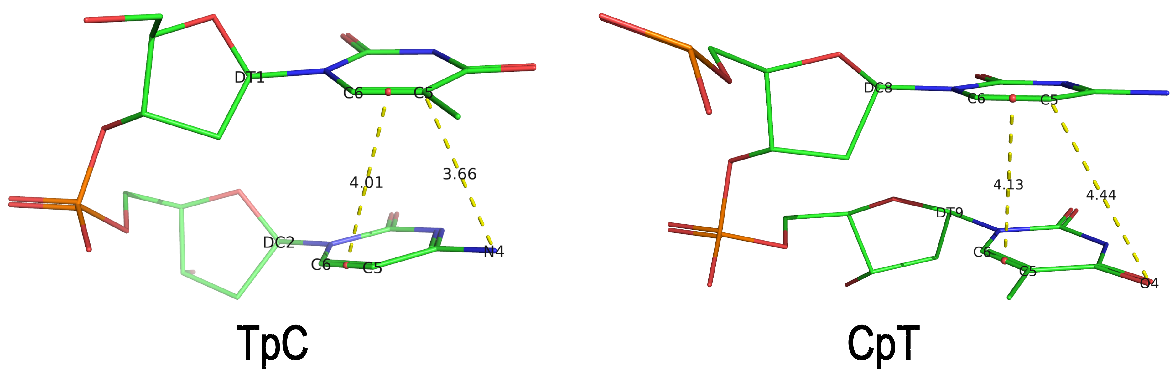
Recently, I read the preprint of Gordan et al. (2025), titled "High-throughput characterization of transcription factors that modulate UVdamage formation and repair at single-nucleotide resolution". In the METHODS section on "Structural analysis of AlphaFold 3 predicted TF-DNA complexes", the authors introduced two geometric parameters to characterize dipyrimidines, as detailed below:
Base-step d22 distance, d64 distance, of dipyrimidines were computed for each base-step per DNA strand using custom PyMOL python scripts74. d22 was defined as the distance in Ångstroms (Å) between the C5-C6 bond midpoints between adjacent pyrimidines. d64 was defined as the Å distance between the 5' pyrimidine's C5 and X4 (either O or N) attached to the 3' pyrimidine's C4.
These d22 and d64 parameters are well-defined and straightforward to calculate (see the figure below for illustrative examples). They can be integrated seamlessly with DSSR's infrastructure, requiring minimal additional coding effort. As a result, I have decided to implement them into DSSR.
For example, in the case of the MyoD bHLH domain-DNA complex (PDB ID: 1mdy), running the following DSSR (v2.7.1) command:
x3dna-dssr -i=1mdy.pdb --json -o=1mdy.json
generates a JSON file (1mdy.json), which contains the following information under the nts section for E.DT1 (connected with E.DC2): "d22": 4.014 and "d64": 3.655."
 The default human-readable output file,
 dssr-torsions.txt, now includes two additional columns for d22 and d64 under the section titled 'Main chain conformational parameters,' as shown below.
          nt        d22     d64
 1     T E.DT1     4.01    3.66
 2     C E.DC2      ---     ---
 3     A E.DA3      ---     ---
 4     A E.DA4      ---     ---
 5     C E.DC5      ---     ---
 6     A E.DA6      ---     ---
 7     G E.DG7      ---     ---
 8     C E.DC8     4.13    4.44
 9     T E.DT9      ---     ---
Note that pseudouridine (Ψ) is excluded from the calculation of d22 and d64 parameters of a dipyrimidine base step.
The implementation of d22 and d64 parameters in DSSR is a clear example of my proactive approach to enhancing the software's functionality. Users are always encouraged to reach out with requests for new features or improvements, as well as to report any bugs or ask questions.
References
- Gordan R, Wasserman H, Chi B, Bohm K, Duan M, Sahay H, et al. High-throughput characterization of transcription factors that modulate UVdamage formation and repair at single-nucleotide resolution. 2025. https://doi.org/10.21203/rs.3.rs-8197218/v1.
 March 2026
 February 2026
Cover image provided by X3DNA-DSSR, an NIGMS National Resource for Structural Bioinformatics of Nucleic Acids (R24GM153869; skmatics.x3dna.org). Image generated using DSSR and PyMOL (Lu XJ. 2020. Nucleic Acids Res 48: e74).
As the developer of DSSR, I am thrilled to see its application in cutting-edge research across multiple disciplines. Below is a list of four recent publications that highlight how DSSR has been utilized, underscoring its versatility and significance in structural bioinformatics.
In the Geng et al. (2025) Nucleic Acids Research (NAR) paper, titled 'Revealing hidden protonated conformational states in RNA dynamic ensembles', DSSR is simply cited as follows:
All bp geometries, hydrogen-bond, backbone, stacking, and sugar dihedral angles were calculated using X3DNA-DSSR [77].
In the preprint by Gordan et al. (2025), titled 'High-throughput characterization of transcription factors that modulate UV damage formation and repair at single-nucleotide resolution', DSSR is cited as follows:
Step base stacking, base pair shift, base pair slide, interbase angle, pseudorotation angle, and sugar puckering classifications of nucleobases were computed using X3DNA-DSSR (v2.5.0)75. Base stacking was defined as the overlapping polygon area in Å2 when projecting the dipyrimidine base ring atoms (excluding exocyclic atoms) into the mean base pair plane76. The sugar ring pseudorotation phase angle of each pyrimidine was also calculated using X3DNA-DSSR as described by Altona, C. & Sundaralingam, M.77 Interbase angle was defined as sqrt(propeller2+buckle2) per the X3DNA-DSSR documentation.
Figure 6: TF Binding Induces Structural Distortion Favorable to UV Dimerization is highly informative, particularly panel (a), which illustrates the ensemble of structural parameters that predispose dipyrimidines to cyclobutane pyrimidine dimers (CPD) or 6-4 pyrimidine-pyrimidones (6-4 PP) formation. DSSR is designed as an integrated software tool, offering a comprehensive suite of structural parameters not found in any other single tool I am aware of. Despite this, the innovative use of DSSR by Gordan et al. exceeds my expectations and demonstrates its versatility.
In the preprint by Kubaney et al. (2025) from the Baker group, titled 'RNA sequence design and protein-DNA specificity prediction with NA-MPNN', DSSR is cited as follows:
On the pseudoknot subset, we evaluate additional structure‐ and reactivity‐based metrics. DSSR v2.3.241 is used to extract the ground‐truth secondary structure from the native crystal structures. For each designed sequence, RibonanzaNet predicts 2A3 reactivity profiles, from which we compute predicted OpenKnot scores (see https://github.com/eternagame/OpenKnotScore)31 using the predicted reactivity together with the DSSR ground truth.
In a recent NSMB paper from the Baker group, titled 'Computational design of sequence-specific DNA-binding proteins', 3DNA is cited as follows:
RIF docking of scaffolds onto DNA targets (DBP design step 1) Structures of B-DNA for each target (Supplementary Table 2) were generated by (1) using the DNA portion of PDB 1BC8 (ref. 60), PDB 1YO5 (ref. 61), PDB 1L3L (ref. 51) or PDB 2O4A (ref. 62) or (2) using the software X3DNA63, followed by a constrained Rosetta relax of the DNA structure.
Please note that 3DNA has been replaced by DSSR. The functionality for constructing B-DNA models, previously provided by 3DNA, is now directly available in DSSR via its fiber and rebuild modules.
In the preprint by Si et al. (2025), titled 'End-to-End Single-Stranded DNA Sequence Design with All-Atom Structure Reconstruction', DSSR is cited as follows:
Since ViennaRNA and NUPACK require secondary structures as input, we used DSSR35 to extract secondary structures from the corresponding ssDNA three-dimensional structures.
The above use cases are merely a sample of how DSSR is utilized in the scientific literature. It is reasonable to state that DSSR has emerged as a de facto standard tool within the field of nucleic acid structural bioinformatics. Overall, DSSR is a mature, robust, and efficient software product that is actively developed and maintained. I am committed to making DSSR synonymous with quality and value. Its unmatched functionality, usability, and support save users significant time and effort compared to alternative solutions.
DSSR is available free of charge for academic users. Additionally, it has been integrated into other high-profile bioinformatics resources, including NAKB, PDB-redo, and N•ESPript.
References
- Geng A, Roy R, Ganser L, Li L, Al-Hashimi HM. Revealing hidden protonated conformational states in RNA dynamic ensembles. Nucleic Acids Research. 2025;53:gkaf1366. https://doi.org/10.1093/nar/gkaf1366.
- Gordan R, Wasserman H, Chi B, Bohm K, Duan M, Sahay H, et al. High-throughput characterization of transcription factors that modulate UV damage formation and repair at single-nucleotide resolution. 2025. https://doi.org/10.21203/rs.3.rs-8197218/v1.
- Kubaney A, Favor A, McHugh L, Mitra R, Pecoraro R, Dauparas J, et al. RNA sequence design and protein–DNA specificity prediction with NA-MPNN. 2025. https://doi.org/10.1101/2025.10.03.679414.
- Glasscock CJ, Pecoraro RJ, McHugh R, Doyle LA, Chen W, Boivin O, et al. Computational design of sequence-specific DNA-binding proteins. Nat Struct Mol Biol. 2025;32:2252–61. https://doi.org/10.1038/s41594-025-01669-4.
- Si Y, Xu Y, Chen L. End-to-end single-stranded DNA sequence design with all-atom structure reconstruction. 2025. https://doi.org/10.64898/2025.12.05.692525.
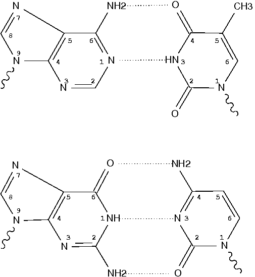
By following DSSR citations, I recently came across the paper by Saon et al. (2025), titled 'Identification and characterization of shifted G•U wobble pairs resulting from alternative protonation of RNA.' This paper provides a detailed analysis of shifted G-U wobble pairs in RNA, characterized by the opposite positioning of G vs. U in the standard G-U wobble pair (see figure below). Conventionally, a G-U wobble has the U located in the major groove, whereas a shifted G-U wobble has the G located in the major groove.
Specifically, the shifted G-U wobble pair involves an H-bond between the N2(G) and N3(U) atoms, which would be donor-donor if U were in its neutral form. There are three ways to rationalize the formation of this H-bond: (1) anionic U as originally proposed by Westhof et al. (2023), (2) U-enolate, and (3) G-imino tautomeric forms as illustrated by Saon et al. (2025). Since the position of the H-atoms cannot be determined from X-ray diffraction and cryo-EM structures, it is not possible (in my understanding) to determine which of these three mechanisms is correct—perhaps it involves a combination of them. What is clear is that the shifted G-U wobble pair is supported by strong experimental evidence from diverse sources. The authors identified 373 high-confidence shifted G-U wobble pairs across four separate structural clusters, spanning all three domains of life.
 Structure of standard and shifted G-U wobble pairs. The examples are taken from PDB entry 8B0X (Fromm et al., 2023) and generated using DSSR and PyMOL. Atom names in the Watson-Crick edges are shown in red and blue for oxygen and nitrogen, respectively. Hydrogen bonds are depicted as dashed lines in magenta. The unusual N2(G)...N3(U) hydrogen bond is marked with a star; it would be donor-donor if U were in its neutral form. The shaded illustration at the bottom is taken from Saon et al., showing shifted G-U wobble pairs in anionic, U-enolate, and G-imino tautomeric forms.
I'm glad to see that DSSR has been used in the analysis, as shown in the following excerpts from the paper.
The selected structures were then characterized by Dissecting the Spatial Structure of RNA (DSSR) software [34]. This step output base pair, hydrogen bond, stacking, glycosidic angle, and sugar pucker information for each structure file.
From the DSSR base pair information, all G•U base pairs were identified and filtered as wobble or non-wobble base pairs. All base pairs called by DSSR as G•U wobbles were considered for the next steps of the analysis as standard wobbles. Any base pairs containing hydrogen bonds between G(N1) and U(O4), as well as G(N2) and U(N3) (see Fig. 1) were binned to shifted wobble base pairs.
From the base pair information extracted from the DSSR characterization output, the non-redundant G•U wobbles were binned based on their location in one of the five secondary structure motifs: (1) inside stem, with one WCF base pair above and one below, (2) terminal, with at least one WCF base pair above, (3) terminal, with at least one WCF base pair below, (4) unstructured, where no WCF base pair is right above or below and the wobble does not occur at the closing base pair of a hairpin loop with a maximum of 10 nucleotides, and (5) inside a loop.
Next, for each of the five members, we retrieved the 3D structure of the 20 residues from the respective pdb files and obtained the underlying secondary structures for each of the five files in dot bracket notation using DSSR [34].
DSSR implements a geometric approach to identify hydrogen bonds, including unconventional donor/acceptor combinations (e.g., the N3-to-N3 hydrogen bond in the hemiprotonated cytosine–cytosine base pair in the i-motif). It is capable of identifying all pairs that actually exist in a given structure, whether they are canonical (Watson-Crick or G-U wobble) or non-canonical. The latter pairs may include normal or modified nucleotides, regardless of their tautomeric or protonation state.
Thus, DSSR detects standard G-U wobble pairs and names them as such ('Wobble'). Moreover, it also detects shifted G-U wobble pairs and previously named them as '~Wobble,' meaning similar to a standard wobble pair. Note that the '~Wobble' designation is based on the geometric approach of DSSR, which involves the cW-W relative orientation of the two bases and a large shear value. It is not limited to wobble pairs between G and U.
After reading the Saon et al. paper, I have revised DSSR to specifically characterize shifted G-U wobble pairs and named them as 'sWobble.' The term 'shifted-Wobble' would be too long for the DSSR text output, and using 's' also reflects the shear parameter, which is key in characterizing wobble pairs. As a concrete example, the following DSSR command
x3dna-dssr -i=8B0X.cif --pair-only --more -o=8B0X-pairs.out
would generate the below output in the file 8B0X-pairs.out. Note the name sWobble, the hydrogen bond N3(imino)*N2(amino)[3.26] with a * to indicate an unusual donor/acceptor combination, and the -2.33 shear value.
607 A.U1086        A.G1099        U-G sWobble     --        cWW  cW-W
     [-171.2(anti) ~C3'-endo lambda=33.9] [-170.0(anti) ~C3'-endo lambda=59.2]
     d(C1'-C1')=11.57 d(N1-N9)=9.60 d(C6-C8)=10.07 tor(C1'-N1-N9-C1')=8.8
     H-bonds[2]: "N3(imino)*N2(amino)[3.26],O4(carbonyl)-N1(imino)[2.64]"
     interBase-angle=26  Simple-bpParams: Shear=-2.23 Stretch=0.69 Buckle=22.1 Propeller=-13.8
     bp-pars: [-2.33   0.13    -0.80   24.83   -7.98   -20.38]
The new DSSR version can automatically detect all 373 high-confidence shifted G-U wobble pairs listed in Table S3 of the Saon et al. paper. It will be released soon. This is yet another example of how DSSR is being actively improved to better serve the research community.
References
- Saon,M.S. et al. (2025) Identification and characterization of shifted G•U wobble pairs resulting from alternative protonation of RNA. Nucleic Acids Research, 53, gkaf575.
- Westhof,E. et al. (2023) Anionic G•U pairs in bacterial ribosomal rRNAs. RNA, 29, 1069–1076.
- Fromm,S.A. et al. (2023) The translating bacterial ribosome at 1.55 Å resolution generated by cryo-EM imaging services. Nat Commun, 14, 1095.
As of v2.5.4-2025jun06, DSSR automatically checks for steric clashes or exact duplicates of residues in an input coordinate file. It reports such issues instead of crashing, and will terminate only if an excessive number of overlaps are detected. An simplified example is shown below, which contains two nucleotides (G#1) on chains 0 and 1, respectively
ATOM      1  OP3   G 0   1      -4.270  51.892  37.186  1.00 27.93           O
ATOM      2  P     G 0   1      -3.834  50.887  37.436  1.00 28.61           P
ATOM      3  OP1   G 0   1      -4.601  49.700  37.549  1.00 27.02           O
ATOM      4  OP2   G 0   1      -4.061  52.011  36.684  1.00 25.80           O
ATOM      5  O5'   G 0   1      -2.906  51.105  38.691  1.00 28.01           O
ATOM      6  C5'   G 0   1      -1.941  52.126  38.781  1.00 26.76           C
ATOM      7  C4'   G 0   1      -1.037  51.914  39.967  1.00 26.12           C
ATOM      8  O4'   G 0   1      -1.822  51.894  41.184  1.00 24.21           O
ATOM      9  C3'   G 0   1      -0.285  50.591  39.988  1.00 25.12           C
ATOM     10  O3'   G 0   1       0.884  50.614  39.172  1.00 26.09           O
ATOM     11  C2'   G 0   1       0.008  50.411  41.462  1.00 26.05           C
ATOM     12  O2'   G 0   1       1.102  51.209  41.880  1.00 27.46           O
ATOM     13  C1'   G 0   1      -1.271  50.952  42.083  1.00 28.40           C
ATOM     14  N9    G 0   1      -2.272  49.904  42.329  1.00 27.27           N
ATOM     15  C8    G 0   1      -3.470  49.733  41.686  1.00 26.55           C
ATOM     16  N7    G 0   1      -4.137  48.712  42.125  1.00 25.36           N
ATOM     17  C5    G 0   1      -3.332  48.176  43.118  1.00 25.64           C
ATOM     18  C6    G 0   1      -3.529  47.056  43.955  1.00 24.98           C
ATOM     19  O6    G 0   1      -4.492  46.284  43.991  1.00 24.56           O
ATOM     20  N1    G 0   1      -2.460  46.862  44.821  1.00 24.78           N
ATOM     21  C2    G 0   1      -1.346  47.639  44.878  1.00 24.96           C
ATOM     22  N2    G 0   1      -0.417  47.298  45.782  1.00 23.72           N
ATOM     23  N3    G 0   1      -1.145  48.689  44.109  1.00 25.74           N
ATOM     24  C4    G 0   1      -2.171  48.901  43.257  1.00 26.32           C
ATOM      1  OP3   G 1   1      -6.437  51.060  40.254  1.00 27.81           O
ATOM      2  P     G 1   1      -5.327  50.209  39.884  1.00 28.55           P
ATOM      3  OP1   G 1   1      -5.668  48.792  39.652  1.00 26.90           O
ATOM      4  OP2   G 1   1      -4.838  51.036  38.808  1.00 25.57           O
ATOM      5  O5'   G 1   1      -4.301  50.297  41.090  1.00 27.94           O
ATOM      6  C5'   G 1   1      -3.427  51.393  41.257  1.00 26.67           C
ATOM      7  C4'   G 1   1      -2.528  51.168  42.443  1.00 26.12           C
ATOM      8  O4'   G 1   1      -3.335  50.964  43.624  1.00 24.16           O
ATOM      9  C3'   G 1   1      -1.648  49.928  42.372  1.00 25.13           C
ATOM     10  O3'   G 1   1      -0.467  50.136  41.599  1.00 26.15           O
ATOM     11  C2'   G 1   1      -1.372  49.649  43.835  1.00 25.96           C
ATOM     12  O2'   G 1   1      -0.375  50.515  44.354  1.00 27.37           O
ATOM     13  C1'   G 1   1      -2.714  50.006  44.458  1.00 28.21           C
ATOM     14  N9    G 1   1      -3.608  48.845  44.581  1.00 27.06           N
ATOM     15  C8    G 1   1      -4.771  48.614  43.895  1.00 26.37           C
ATOM     16  N7    G 1   1      -5.340  47.496  44.226  1.00 25.18           N
ATOM     17  C5    G 1   1      -4.502  46.957  45.190  1.00 25.44           C
ATOM     18  C6    G 1   1      -4.599  45.755  45.923  1.00 24.77           C
ATOM     19  O6    G 1   1      -5.480  44.892  45.864  1.00 24.39           O
ATOM     20  N1    G 1   1      -3.532  45.594  46.796  1.00 24.63           N
ATOM     21  C2    G 1   1      -2.504  46.469  46.949  1.00 24.81           C
ATOM     22  N2    G 1   1      -1.560  46.145  47.845  1.00 23.58           N
ATOM     23  N3    G 1   1      -2.396  47.594  46.280  1.00 25.56           N
ATOM     24  C4    G 1   1      -3.422  47.779  45.423  1.00 26.12           C
Running DSSR on the above coordinates will show the following output:
[i] 0.G1 and 1.G1 in clashes: min_dist=0.57
where min_dist refers to the minimum distance between heavy atoms of the two nucleotides.
The clash-detection feature in DSSR was added in response to the bioRxiv preprint by Kretsch et al. (2025), titled "Assessment of nucleic acid structure prediction in CASP16" (https://doi.org/10.1101/2025.05.06.652459), which noted that in some predicted RNA models submitted to CASP16, multiple models were not properly delineated with MODEL/ENDMDL in PDB format or _atom_site.pdbx_PDB_model_num in mmCIF format. I communicated with the authors, who kindly provided the PDB files to help debug the issue. For more details, see the blog post Improving DSSR through extreme cases from early June 2025 at https://x3dna.org/highlights/improving-dssr-through-extreme-cases.
The bioRxiv paper by Kretsch et al. was recently published in Proteins: Structure, Function, and Bioinformatics. The relevant citation to DSSR is in Section 2.8 | Secondary Structure Analysis, as follows:
Secondary structures were extracted from CASP16 models with DSSR (v1.9.9-2020feb06) [47]. Some models, in particular due to large clashes, could not be processed by DSSR (Table S1). The base-pair list was extracted from the table in the output file directly because the dot-bracket structure produced by DSSR, in particular for multimers, contained errors. The canonical base pairs were defined as those labeled as Watson-Crick-Franklin (WC) and wobble base pairs (hereafter referred to as ‘base pairs’ or ‘pairs’). All other base pairs are defined as non-canonical base pairs and analyzed separately. Crossed base pairs (pseudoknots) were defined as non-nested canonical base pairs, that is, any canonical base pair (i,j) for which another canonical base pair (k,l) existed with i < k < j < l or k < i < l < j. Singlet base pairs were defined as any canonical base pair that was not part of a stem, that is, (i,j) such that there was no neighboring canonical base pair between i + 1 and j − 1 or between i − 1 and j + 1. Intermolecular base pairs were identified as any canonical base pair between nucleotides in different chains.
It is worth noting that DSSR is actively supported, and I always strive to respond to users’ questions via email or (preferably) on the 3DNA Forum quickly and concretely. If you have any questions about DSSR or need clarifications, please feel free to contact me. Additionally, I monitor 3DNA/DSSR citations in the literature and proactively address issues that come to my attention when necessary.
I recently came across the paper by Zurkowski et al. (2025), titled "Detecting polynucleotide motifs: Pentads, hexads, and beyond.". The authors introduce LinkTetrado, a software tool that is described as "the first fully automated method for detecting polyadic motifs in the three-dimensional structures of nucleic acids." I am somewhat surprised by this claim, as I believe it overlooks the 2015 DSSR paper, which includes a dedicated section on "Higher-order coplanar base associations (multiplets)" as shown below:
DSSR defines multiplets as three or more bases associated in a coplanar geometry via a network of hydrogen-bonding interactions. Multiplets are identified through inter-connected base pairs, filtered by pair-wise stacking interactions and vertical separations to ensure overall coplanarity (Supplementary Figures S1, S3, S4 and S7). The abundant A-minor motifs (33) (types I and II, Supplementary Figures S3, S4 and S7) are base triplets, the smallest multiplet. The G-tetrad motif, where four guanines are associated via four pairs in a square planar geometry, is another special case of a multiplet.
In fact, DSSR multiplets are all-encompassing, including pentads, hexads, heptads, octads, etc.
The DSSR User Manual has extensive discussions (see Section 3.2.4 "Multiplets (higher-order coplanar base associations)") and several examples of multiplets, including:
- Figure 8: The GUA triplet auto-identified by DSSR in PDB entry 1msy.
- Figure 12: Base pentad (AUAAG) auto-identified by DSSR in PDB entry 1jj2. The five nts (A306,U325,A331,A340,G345) are all within the 23S rRNA.
DSSR can successfully identify the multiplets reported in the Zurkowski et al. paper, although there may be minor differences due to variations in cutoffs and definitions. For instance, using PDB ID 6w9p (shown in Fig. 7F of the Zurkowski et al. paper), DSSR can perform the following:
x3dna-dssr -i=6w9p.pdb -o=6w9p.out
x3dna-dssr -i=dssr-multiplets.pdb --select-model=4 -o=G4T3.pdb
The relevant portions of DSSR output (6w9p.out) are shown below:
List of 4 multiplets
   1 nts=4 GGGG A.DG4,A.DG10,A.DG16,A.DG22
   2 nts=4 GGGG A.DG5,A.DG11,A.DG17,A.DG23
   3 nts=4 GGGG A.DG7,A.DG13,A.DG19,A.DG25
   4 nts=7 GTGTGTG A.DG6,A.DT9,A.DG12,A.DT15,A.DG18,A.DT21,A.DG24

...
2 dssr-multiplets.pdb -- an ensemble of multiplets
DSSR can further render the extracted G4T3.pdb into the following image using PyMOL:

DSSR has far more to offer than meets the eye. See the DSSR User Manual and the practical guide to DSSR-PyMOL integration for more details.
References
Lu,X.-J. et al. (2015) DSSR: an integrated software tool for dissecting the spatial structure of RNA. Nucleic Acids Res, gkv716.
Zurkowski,M. et al. (2025) Detecting polynucleotide motifs: Pentads, hexads, and beyond. PLoS Comput Biol, 21, e1013633.
By following citations related to 3DNA/DSSR, I recently discovered the paper “Computational Insights into the Structural and Energetic Properties of an A/C stacked Three-Way DNA Junction” by Singh et al. (2025), published in the new journal Computational and Structural Biotechnology Reports. The study investigates the conformational dynamics, stability, and compactness of a DNA three-way junction (3WJ) through molecular dynamics (MD) simulations.
3WJs are the simplest and most common branched nucleic acids, consisting of three double-helical stems (A, B, and C), connected at a junction point. Two of these stems can be coaxially stacked, forming either an A/B-stacked or A/C-stacked structure. The Singh et al. study utilized the A/C-stacked 3WJ PDB entry 1snj as the starting point for their simulations. DSSR efficiently identifies the three stems and two helices, with one helix formed by the coaxial stacking of two stems.
The entire section '2.2. Conformational Analysis of the DNA Junction' from the Singh et al. paper has been quoted below. I am delighted to see 3DNA/DSSR referenced in this manner.
In this work, 10 snapshots were gathered at periodic intervals of 100 ns from the 1000.0 ns molecular dynamics simulation trajectory. We have utilized the X3DNA program [48,49,50] to analyze, recreate, and visualize three-dimensional nucleic acid structures. X3DNA is capable of both the antiparallel and the parallel double-helices, the single-stranded structures, the triplexes, the quadruplexes, as well as the other intricate tertiary motifs which is present within the DNA and the RNA structures. This analysis procedures classify and identify all the fundamental interactions and also categorize the suitable base-pair-steps double-helical properties. This program uses a reference frame for the explanation of the nucleic acid basepair geometry as well as a rigorous matrix-based approach to compute the local conformational- parameters and also reconstruct structure using these parameters. The helicoidal parameters and the torsion-angle parameters are essential in comprehending folding and the rotation of the bases during the dynamical pathway.
Although there are specialized software tools designed for analyzing MD trajectories, the features available in DSSR appear to be adequate for applications like those described in the Singh et al. paper. DSSR has no external dependencies, is easy to use, and provides a more detailed characterization of nucleic acid structures than other tools. Furthermore, it is actively maintained and supported. If you have any questions or feature requests, feel free to reach out—I am here to help!
For completeness, I’ve included the relevant parts from the DSSR User Manual in this post.
The DSSR --nmr (or --md) option automates the analysis of an ensemble, such as NMR structures in the PDB or snapshots from MD simulations. The input coordinates file must be in either the classic PDB format where each model is delineated by MODEL/ENDMDL tags, or the mmCIF format where each ATOM/HETATM record has an associated model number.
The --json option makes it easy to parse the output of multiple models pragmatically. In addition to NMR structures, trajectories from MD simulations can also be processed. Popular MD packages (AMBER, GROMACS, CHARMM, etc.) all have their own specialized binary formats for trajectories. By design, DSSR does not work on these binary files. They must be converted to the standard PDB or mmCIF format to be analyzed by DSSR. The combination of --nmr and --json makes DSSR directly accessible to the MD community.
See also the threads "Do I need gromacs to use dnaMD for simulations?"" and "Update of do_x3dna package" on the 3DNA Forum.
References
Singh,A. et al. (2025) Computational Insights into the Structural and Energetic Properties of an A/C stacked Three-Way DNA Junction. Computational and Structural Biotechnology Reports, 100055.
Recently, I noticed that a user had uploaded a file to the website "DSSR-enabled Innovative Schematics of 3D Nucleic Acid Structures with PyMOL", which DSSR reported as 'no nucleotides found.' Upon visualizing it in PyMOL, the structure appeared to be a single-stranded RNA. Further investigation revealed that while the uploaded file was in PDB format, it did not adhere to the standard naming conventions for nucleotides typically used in RCSB PDB entries. For instance, an A nucleotide extracted from the file had its exocyclic amino group named as N553 instead of the conventional N6 (see below).
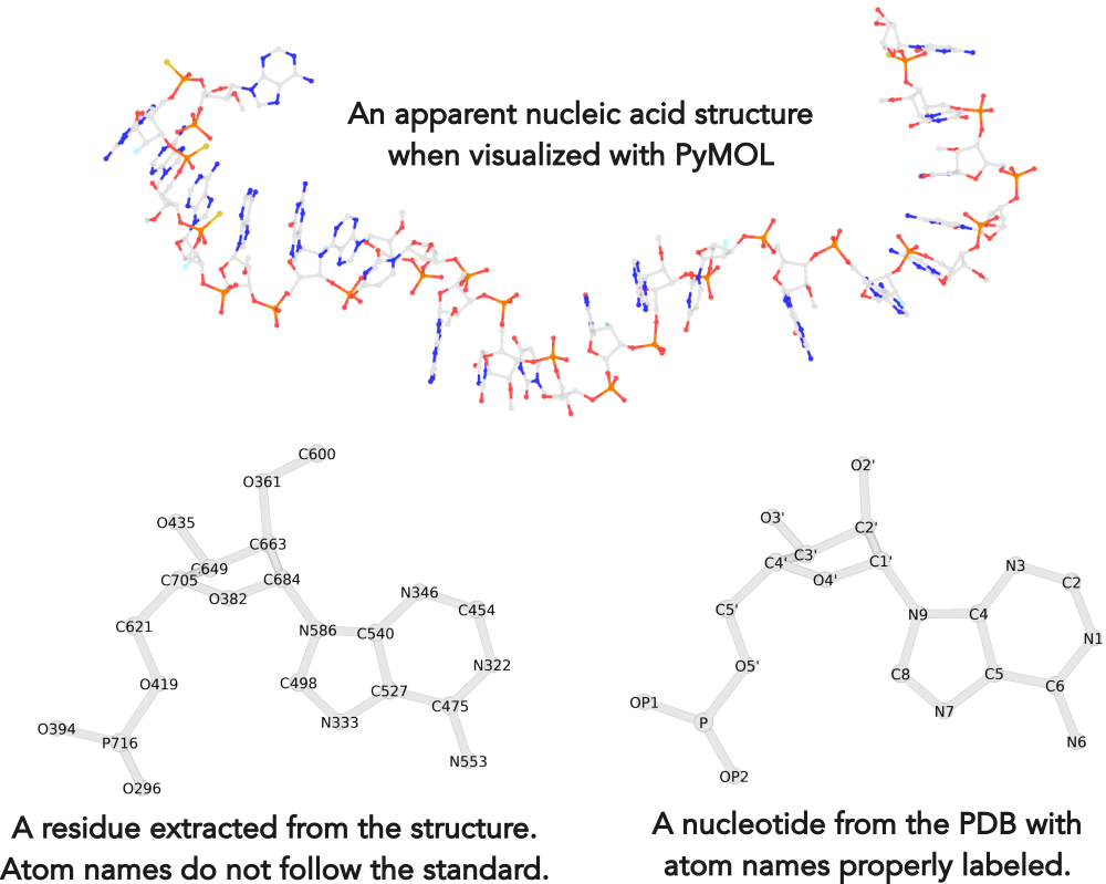
Following 3DNA, DSSR uses the atomic coordinates and standard names of base-ring atoms to identify a nucleotide. All known nucleotides share a common six-membered pyrimidine ring, with atoms named consecutively (N1, C2, N3, C4, C5, C6), and purines include three additional atoms (N7, C8, N9). See below for the standard names in Watson-Crick base pairs.
Without proper names for base ring atoms, DSSR is unable to identify nucleotides, resulting in the input structure being reported as 'no nucleotides found.' The same principle applies to amino acids in protein structures, such as specific naming conventions for amino nitrogen (N), carbonyl carbon (C), and alpha carbon (CA).
See also the blog posts "Mapping of modified nucleotides in DSSR" and "Name of base atoms in PDB formats".
By following DSSR citations, I recently noticed a bioRxiv preprint, titled "Assessment of nucleic acid structure prediction in CASP16" by Kretsch et al. The portion where DSSR is mentioned is as follows:
Secondary structures were extracted from CASP16 models with DSSR (v1.9.9-2020feb06). Some models, in particular due to large clashes, failed to run (Supplemental Table 1). The base-pair list was extracted from the table in the output file directly because the dot-bracket structure produced by DSSR, in particular for multimers, can contain errors.
While pleased to see DSSR cited in this significant study, I am concerned about the reported issues and would like to investigate the specific structures and error messages encountered. To better understand the problems and potentially find solutions, I have reached out to the authors for further details. Here is the message I sent initially:
You said DSSR failed to run on some models with large clashes. Could you please share the specific models and the error messages you encountered? I would also be interested in seeing the exact errors you observed in the DSSR-derived DBN for multi-mers. It would be a great opportunity for me to improve DSSR in this area, which would benefit both your group and the broader community. If you are willing to share them, please provide details—preferably on the **public 3DNA Forum**. Don’t hesitate to share openly any bugs or limitations you’ve encountered with DSSR.
The authors responded promptly and provided detailed information about the specific models and error messages encountered. After several
iterations, I successfully resolved the issues and released an updated version of DSSR, namely v2.5.4-2025jun04. You can find the release notes
here. This experience underscores the importance of proactively engaging with the community to enhance the functionality and reliability of a software tool.
In this blog post, I aim to share the specifics of these issues and the steps taken to address them. For ease of reading, I have formatted the response/feedback from the authors in red block quotes, and my enquiries/comments in blue. The beginning round of correspondence is as below.
Do note, the predictors in casp submit some truly atrocious models --- eg 14 atoms all at the exact same x-y-z coordinate. These errors would be with his v1.9.9-2020feb06 install though not your latest version. Would you still like them?
Yes, I would like to see how DSSR behaves with these models. Ideally, it should not crash, but output some warning messages. Only through such testing can we improve the robustness of DSSR. Overall, the more feedback I get, the better.
Buffer overflow bug in DSSR
Most of errors I had with dssr were due to clashes and all zero xyz predictions by predictors, for all of which dssr did not give an error message when dssr failed. There was a case where the prediction looked reasonable but dssr failed with the error message `dssr error*** buffer overflow detected ***`. Please see attached for the 2 pdbs that gave this error.
The two PDB files I received were R1283v3TS294_1o and R1283v3TS294_2o, as listed in Supplementary Table 1: "List of unscored models," with the "Reasons" column indicating a dssr error*** buffer overflow detected ***. I immediately acknowledged receipt of these files, as shown in the following message:
Thank you for sending me the two PDB files which caused DSSR to fail. I can verify the issue and will try to fix the bug ASAP. I'll keep you posted.
Using these data files, I was able to quickly fix the buffer overflow bug. The following is my response to the authors within one day after receiving the files:
With your sample PDB files, I have traced the issue that caused DSSR to fail. The bug was due to a 53-way (`R1283v3TS294_1o`) and 40-way (`R1283v3TS294_2o`) junction loops which are far from the norm. DSSR sets a default limit for the summary line for each loop which is more than sufficient for all normal PDB entries, but falls short for these unusual cases, leading to out of array boundaries. See the attached DSSR output after the bug fix for more details.
This is a clear example where user feedback is crucial for improving the software, which makes it better serve the community.
Zero xyz coordinates and large clashes
After fixing the out-of-bound bug, I also requested other problematic predicted models from the authors, as shown in the following message:
Along the line, please provide the sample PDB files:
- with zero xyz predictions -- I am curious to see what it looks like.
- where the DSSR-derived DBN is problematic for multi-mers
After solving these issues, I will release a new version of DSSR that would make your analysis more straightforward, and benefit other users as well.
The authors responded with the following message:
Thanks for looking into this. Here are some more examples with superimposed structures, large clash, and all zero xyzs in the zip file.
The ZIP file (error_examples.zip) contains three folders (all_zero_xyz, clash and superimposed), each with some problematic models in PDB format. Once again, I promptly acknowledged receipt of the files and was able to reproduce the reported issues.
Garbage in, garbage out. Given these problematic models, one should not expect DSSR to extract any meaningful information from them. Nonetheless, I am committed to enhancing the software so that it can handle such cases more effectively by providing clear error messages and terminating gracefully rather than crashing.
After several days of thinking, elaboration, intensive coding, and testing, I solved the problems. I then communicated the results to the authors in the following detailed message:
Thanks for the sample PDB files (`error_examples`) with all zero XYZ coordinates, large clashes, and superimposed structures. They helped me to understand the issues, think in context, and find solutions. Let's look them one by one:
1. `all_zero_xyz`: These two files `R1211TS159_1` and `R1211TS159_2` have identical contents, except for the MODEL IDs (1 and 2, respectively). Atoms with all-zero XYZ coordinates are a special case of duplicated coordinates. This has led me to implement a check for duplicated coordinates in an input file. The revised DSSR now reports duplicated coordinates and their corresponding atoms, and it quits if the number of duplicated atoms exceeds a certain threshold. For `R1211TS159_1`, the revised DSSR output would be as below:
   1 [e] xyz repeated 1904 times:[0.000      0.000      0.000]   1509-P@0.G1   3412-C6@0.C90
[w] no-of-repeats=1 max-freq=1904
...too many duplicates... quit!
2. `clash`: Both files `R1250TS208_1o` and `R1250TS417_1o` contain multiple models, as visible in PyMOL. Each PDB file uses a single MODEL/END pair to include all its models. This setup is akin to an NMR ensemble but without MODEL/ENDMDL delimiters, which leads to clashes when analyzed together. I have revised DSSR to explicitly check for such clashes and terminate execution if too many are detected. Using `R1250TS208_1o` as an example, the DSSR output would be as below:
[i] 0.G1 and 1.G1 in clashes: min_dist=0.57
[i] 0.G1 and 3.G1 in clashes: min_dist=0.35
[i] 0.G1 and 4.G1 in clashes: min_dist=0.41
...too many clashes... quit!
The above list contains only three of the many clashes detected in this file. One can notice immediately the G1 nucleotides from chains `0`, `1`, `3`, and `4` are in clashes (see the attached file `clashes_208.pdb`, which contains only G1 nucleotides from the four chains).
3. `superimposed`: The five example files (`R1283v3TS304_1o` ... `R1283v3TS304_5o`) have similar issues as the clash cases. Running the revised DSSR on `R1283v3TS304_1o` would produce the following output:
[i] 0.A1 and 2.A1 in clashes: min_dist=0.74
[i] 0.A1 and 3.A1 in clashes: min_dist=0.78
[i] 0.A1 and 4.A1 in clashes: min_dist=0.56
...too many clashes... quit!
Here A1 nucleotides from chains `0`, `2`, `3` , and `4` are in clashes (see the attached `superimpose-1.pdb`).
How the `clash` and `superimposed` categories are supposed to be different? They look similar to me.
Overall, the `error_examples` (in `all_zero_xyz`, `clash`, and `superimposed`) pose problems because they do not contain valid DNA/RNA structures as a whole. DSSR cannot extract meaningful information from these files. However, the revised DSSR explicitly highlights these issues, saving users from spending time on invalid data. Do these DSSR revisions make sense to you?
In the end, I am glad to receive the following feedback from the authors:
Thanks, these revisions all make sense! The examples I sent on clashes and superimposed were actually similar and I think the error output makes sense as well.
Final thoughts
This blog post offers an in-depth look at my efforts to enhance DSSR. As the developer of this software product, I am deeply committed to ensuring its quality and usability. I extend my gratitude to the authors for their valuable feedback and assistance in resolving these issues. In return, the updated version of DSSR (v2.5.4-2025jun04) should not only streamline their workflow but also benefit the broader user community.
For those who read through this lengthy post, I want to emphasize that DSSR is actively supported: I am here to listen and help. Any questions related to its use, bug reports, or feature requests are warmly welcomed on the 3DNA Forum. As I’ve mentioned before, please don’t hesitate to share any negative experiences or bugs with DSSR—just ensure to provide specific details so others can reproduce the issue. I will address these concerns as soon as I’m aware of them and will frankly acknowledge any mistakes I may have made. My goal is for DSSR to be a reliable software tool that the community can trust and build upon.
References
Kretsch,R.C. et al. (2025) Assessment of nucleic acid structure prediction in CASP16. bioRxiv; https://doi.org/10.1101/2025.05.06.652459.
In DSSR, the --frame option allows users to reorient a nucleic acid structure using the standard base reference frame (see Olson et al., 2001). This option can be applied not only to an individual base frame but also a base-pair frame, or the middle frame between two bases or base pairs. These variations facilitate the alignment of nucleic acid structures for a wide range of comparative analyses. In this blog post, I will demonstrate how to use the --frame option with concrete examples, enabling readers to apply this unique DSSR feature to their own projects.
The standard base reference frame
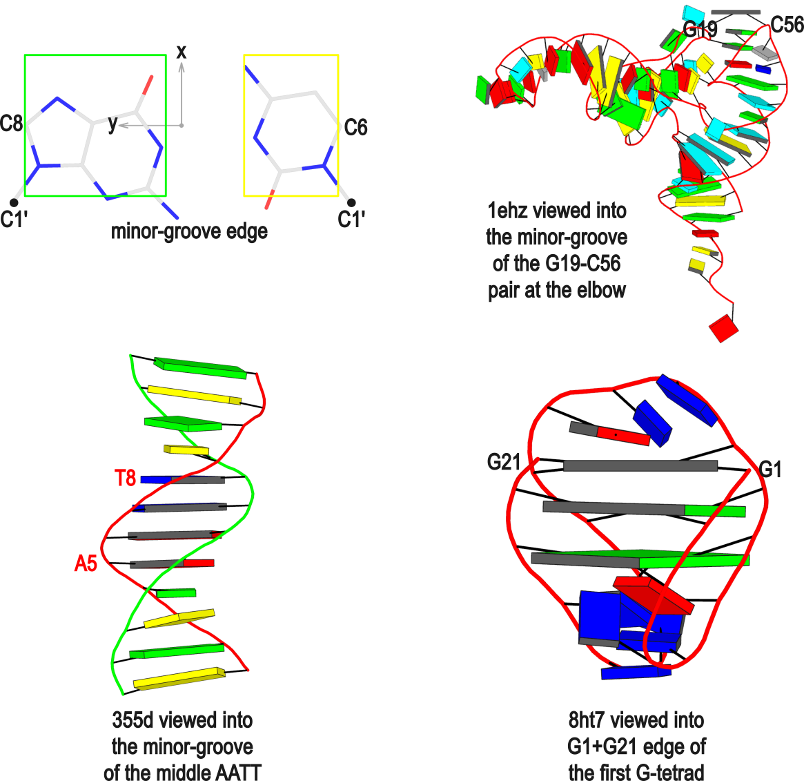
The standard base reference frame is derived from an idealized Watson-Crick base pairing geometry (top-left, figure below). The x-axis points in the direction of the major groove along what would be its pseudo-dyad axis—that is, the perpendicular bisector of the C1'...C1' vector spanning the base pair. The y-axis runs along the long axis of the idealized base-pair in the direction of the sequence strand, parallel to the C1'...C1' vector, and is displaced so as to pass through the intersection between the (pseudo-dyad) x-axis and the vector connecting the pyrimidine Y(C6) and purine R(C8) atoms. The z-axis is defined by the right-handed rule. For right-handed A- and B-DNA, the z-axis accordingly points along the 5' to 3' direction of the sequence strand.
Typical usages of the --frame option
Using the classic B-DNA dodecamer PDB entry 355d as an example, DSSR can be run with the --frame option as follows:
#             1...5..8....
# chain A: 5'-CGCGAATTCGCG -3'
# chain B: 3'-GCGCTTAAGCGC -5'

# reorient 355d in the reference frame of C1 on chain A
x3dna-dssr -i=355d.pdb --frame=A.1 -o=355d-b1.pdb

# reorient 355d in the frame of the Watson-Crick pair C1-G24
x3dna-dssr -i=355d.pdb --frame=A.1:wc -o=355d-bp1.pdb

#  ... with the minor-groove of pair C1-G24 facing the viewer
x3dna-dssr -i=355d.pdb --frame=A.1:wc-minor -o=355d-bp1-minor.pdb

# with the minor-groove of the middle AATT tract facing the viewer
x3dna-dssr -i=355d.pdb --frame='A.5:wc-minor A.8:wc' -o=355d-AATT-minor.pdb

# Rendered in cartoon-blocks with base-pair blocks, and black minor-groove
# Load 355d-AATT-minor.pml into PyMOL (bottom-left, figure above)
x3dna-dssr -i=355d-AATT-minor.pdb --cartoon-block --block-file=wc-minor -o=355d-AATT-minor.pml
The abbreviated notation A.1 refers to nucleotide numbered 1 (as indicated in the coordinates file) on chain A. Here, it denotes C1, as shown at the top of the listing. Similarly, A.5 and A.8 correspond to nucleotides A5 and T8 on chain A, respectively. In most cases, such as with 355d, the combination of chain identifier and residue number is sufficient to uniquely identify a nucleotide. More generally, other information such as model number or insertion code may be needed to specify a particular nucleotide.
In the above listing, wc after the colon (for example, A.1:wc) specifies the Watson-Crick base pair that the corresponding nucleotide participates in. Meanwhile, minor transforms the structure so that the minor-groove of the base (or base pair, or step) faces the viewer. The keywords wc and minor are settings that influence the construction or view of the frame. Case or order does not matter for these keywords as long as there is a match—for example, minor+wc works the same as wc-minor.
Two other examples combining the --frame option with cartoon-block representations
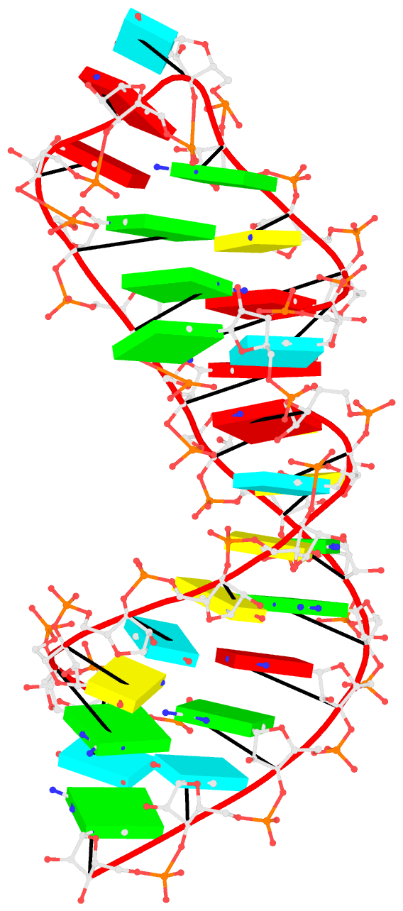
The intuitive geometric meaning of the standard base reference frame combined with the DSSR-enabled cartoon-block representation allows for an enhanced understanding of intricate structural features. In the top-right panel of the figure above, we see the classic yeast phenylalanine tRNA (PDB entry 1ehz) viewed into the minor-groove of the pseudo-knotted G19-C56 pair at the elbow of the L-shaped tertiary structure. The stacking interactions of the purines at the top-right of the panel are clearly visible in this view. In the bottom-right panel, an anti-parallel G-quadruplex from PDB entry 8ht7 is shown. The G-tetrads are automatically identified and rendered as square blocks, all with DSSR. This representation makes the chair conformation of the three-layered anti-parallel G-quadruplex crystal clear. The DSSR commands used are listed below:
# yeast tRNA (1ehz)
x3dna-dssr -i=1ehz.pdb --frame=A.19:wc-minor -o=1ehz-elbow.pdb
x3dna-dssr -i=1ehz-elbow.pdb --cartoon-block --block-file=wc-minor -o=1ehz-elbow.pml

# anti-parallel chair-shaped G-quadruplex (8ht7)
x3dna-dssr -i=8ht7.pdb --select=nts -o=8ht7-nts.pdb  # extract nucleotides, ignore amino acids
# reorient 8ht7 in the frame of the G-tetrad involving G1, in edge view
x3dna-dssr -i=8ht7-nts.pdb --frame=A.1:G4-minor -o=8ht7-Gtetrad.pdb
x3dna-dssr -i=8ht7-Gtetrad.pdb --block-cartoon --block-file=G4-minor -o=8ht7-Gtetrad.pml
References
Olson,W.K. et al. (2001) A standard reference frame for the description of nucleic acid base-pair geometry. Journal of Molecular Biology, 313, 229–237.
The 3DNA suite includes the mutate_bases program, which, as its name suggests, mutates bases while maintaining the backbone conformation. This feature was incorporated into the suite following user feedback and has been utilized in several studies before being formally published in the Li et al. (2019) paper. A key advantage is that the mutation process preserves both the geometry of the sugar-phosphate backbone and the base reference frame, encompassing position and orientation. Consequently, re-analyzing the mutated model yields identical base-pair and step
parameters as those of the original structure.
In DSSR, the standalone mutate_bases program has become the mutate sub-command with enhanced functionality and improved usability, as documented in the User Manual. The mutate module allows users to perform base mutations efficiently and effectively by taking advantage of the powerful DSSR analysis engine.
To further expand the modeling capabilities of the DSSR, v2.5.3 introduced the --mutate-type option to allow for backbone mutations, based on the base reference frame. Furthermore, the target can be any fragment, regardless of length or composition, rather than just a single nucleotide. When combined with the rebuild module, this feature significantly enhances DSSR’s ability to model nucleic acid structures.
Here is an example of modeling PDB entry 1msy, a 27-nt structure (1msy.pdb) that mimics the sarcin/ricin loop from E. coli 23S ribosomal RNA.
x3dna-dssr analyze -i=1msy.pdb --ss --rebuild -o=1msy-expt.out
mv dssr-ssStepPars.txt 1msy-step.txt
x3dna-dssr rebuild --backbone=RNA --par-file=1msy-step.txt -o=1msy-step.pdb

x3dna-dssr -i=1msy.pdb --select-resi='A 2654' -o=1msy-A2654.pdb
x3dna-dssr -i=1msy.pdb --select-resi='A 2655' -o=1msy-G2655.pdb
x3dna-dssr -i=1msy-A2654.pdb --frame=2654 -o=frame___A.pdb
x3dna-dssr -i=1msy-G2655.pdb --frame=2655 -o=frame___G.pdb

x3dna-dssr mutate -i=1msy-step.pdb --entry='num=8 to=A; num=9 to=G' -o=1msy-C2endo.pdb --mutate-part=whole
x3dna-dssr --connect-file -i=1msy-C2endo.pdb -o=1msy-C2endo-cnt.pdb --po-bond=5.0
- The
analyze step uses options --ss and --rebuild to generate the file dssr-ssStepPars.txt (containing base-step parameters), which is then renamed to 1msy-step.txt. The rebuild step employs 1msy-step.txt to construct a structure (1msy-step.pdb) with regular C3'-endo sugar RNA backbone conformation. Note that the rebuilt structure has nucleotides numbered from 1 to 27, while in the PDB 1msy, they correspond to 2647 to 2673, respectively.
- However, the A2654 and G2655 dinucleotides in 1msy are actually in C2'-endo sugar conformation, creating the S-shaped structure around the GpU platform. The above rebuilt structure does not reflect this distortion. So we extract A2654 and G2655 with
--select-resi and then put each in its standard base reference frame, named frame___A.pdb and frame___G.pdb, respectively.
- Now we mutate A8 and G9 in the rebuilt structure
1msy-step.pdb to A and G with option --mutate-part=backbone to ensure the backbone conformations are changed according to those in frame___A.pdb and frame___G.pdb, respectively. The resulting structure is named 1msy-C2endo.pdb. Now the S-shape around the GpU platform is preserved, even though the backbone are not always covalently connected, due to large O3'(i-1) to P(i) distances between neighboring nucleotides. The last step is to generate CONECT records with --connect-file option to connect the backbone atoms explicitly, resulting in more smooth backbone cartoon representation in PyMOL as shown below.
As noted in the Li et al. (2019) paper, users can optimize this approximate backbone connection using Phenix, while keeping the base atoms fixed. The 3DNA-Phenix combination leads to a model where the base geometry strictly follows the parameters prescribed in the user-specified file, and the backbone is regularized with improved stereochemistry and a ‘smooth’ appearance in ribbon representation.
There are other variants of the DSSR mutate module, including for building Z-DNA backbones. However, the above example is sufficient to demonstrate the power of the integrated approach enabled by DSSR for the analysis and modeling of nucleic acid structures. See the DSSR User Manual for more details.
References
Li,S. et al. (2019) Web 3DNA 2.0 for the analysis, visualization, and modeling of 3D nucleic acid structures. Nucleic Acids Res., 47, W26–W34.
Background and motivation
In late 2021, I came across the thread titled "create a 26 bp RNA from a 13 bp
system" on the PyMOL mailing list. The thread began with a user asking:
I have an RNA duplex with 13 base-pairs (attached). Is it possible to duplicate this system and then fuse the two molecules to create a 26 base-pair long system using the pymol.
The message is both concise and clear. The attached 13 base-pair RNA duplex (named model.pdb) makes the task easier to understand. An expert PyMOL user responded quickly, providing a set of suggested PyMOL commands along with warnings about the complexity of the task.
No, not automatically. Your RNA is very distorted from the standard A-form. I doubt any modeling program can accurately extend such a distorted helix. Maybe someone else will prove me wrong. ... You can align the terminal base pairs manually through a series of commands. If you try by dragging one copy relative to another, you will wind up pulling out all of your hair. The commands and patience will keep you out of the mad house.
DSSR offers unique capabilities to automatically manipulate nucleic acid structures. It also enables the duplication of an RNA duplex, as specifically requested by the original poster. In my initial response to the thread, I provided a DSSR-based solution for duplicating the RNA duplex without detailed explanations, aiming to confirm whether the result met the user's needs. The feedback was positive, as indicated below:
Thanks for proving me wrong. Congratulations on your duplicated model! Please share the commands that you used with DSSR to generate the duplicated helix. --- from the PyMOL responder
Thanks a lot for your help. The model you have duplicated is exactly what I am looking for (checked it with VMD). Unfortunately I do not have access to DSSR-Pro. Is there any way that I can reproduce your procedure with x3dna-dssr? I need to create different numbers of duplicates (2,4,6,5,8) for different systems and this will be very helpful. --- from the original poster
During that period (near the end of 2021), I was facing a funding gap. To address this challenge, we decided to license DSSR through Columbia Technology Ventures (CTV) and introduced a Pro version of DSSR for commercial users and academic institutions, providing advanced modeling features and dedicated support. Note that DSSR Pro Academic licenses entail a one-time fee of $1,020. The software can be installed on Windows, macOS, or Linux. While not explicitly included in the license agreement, I provide direct support to Pro license users via email, phone, or Zoom whatever convenient to help address their issues. I care about user experience, especially for those who invest in the Pro version.
Following user feedback, I shared detailed instructions on duplicating an RNA duplex using DSSR Pro. Gratefully, the original poster purchased a DSSR Pro Academic license and successfully duplicated the RNA helix. Later, we communicated via email to assist with other related tasks. This experience underscored the importance of engaging with the scientific community and addressing user needs to drive software development and adoption.
Detailed instructions
With funding from grant R24GM153869, I have transferred many DSSR Pro features into the free DSSR Academic version to better serve the scientific community. Included below are detailed step-by-step commands script for duplicating an RNA duplex using either DSSR Pro or the free DSSR Academic v2.5.2. The script runs instantaneously in a terminal window.
x3dna-dssr tasks -i=model.pdb --frame-pair=last -o=model1-ref-last.pdb

x3dna-dssr fiber --seq=GG --rna-duplex -o=conn.pdb
x3dna-dssr tasks -i=conn.pdb --frame-pair=first --remove-pair -o=ref-conn.pdb

x3dna-dssr tasks --merge-file='model1-ref-last.pdb ref-conn.pdb' -o=temp1.pdb

x3dna-dssr tasks -i=temp1.pdb --frame-pair=last --remove-pair -o=temp2.pdb
x3dna-dssr tasks -i=model.pdb --frame-pair=first -o=model1-ref-first.pdb

x3dna-dssr tasks --merge-file='temp2.pdb model1-ref-first.pdb' -o=duplicate-model.pdb

x3dna-dssr --order-residue -i=duplicate-model.pdb -o=temp3.pdb
x3dna-dssr --renumber-residue -i=temp3.pdb -o=temp4.pdb
x3dna-dssr --connect-file -i=temp4.pdb -o=RNA-duplicate.pdb
The procedure is essentially the same as the one used in "Building extended Z-DNA structures with backbones using DSSR". For completeness, I have included detailed
explanations for each step here as well.
-
Setting Up the Reference Frame:
- The first command places the 13 base-pair RNA duplex (
model.pdb) into the reference frame of its last base pair, resulting in model1-ref-last.pdb.
-
Creating the Fiber Connector:
- The
fiber model is constructed using an RNA duplex (--rna-duplex) with the sequence GG on the leading strand (conn.pdb). This connector is oriented into the reference frame of its first base pair.
- The first base pair is removed. Thus, the resulting coordinate file,
ref-conn.pdb, contains only one pair.
- Note: The sequence GG serves as a placeholder. It can be replaced with any other two bases: for instance, changing
--seq=GG to --seq=AA. Moreover, using --seq=GA10G allows for creating a linker with 10 adenines.
-
Merging PDB Files:
- The two PDB files,
model1-ref-last.pdb and ref-conn.pdb, share a common reference frame and are merged into a single file named temp1.pdb.
-
Adjusting the Reference Frame:
- The merged file (
temp1.pdb) is then aligned with the last base pair, which is subsequently removed to produce temp2.pdb. This completes the role of the GG fiber connector.
-
Reorienting the RNA Duplex:
- The original 13 base-pair RNA duplex (
model.pdb) is reoriented into the reference frame of its first base pair, generating model1-ref-first.pdb.
-
Final Merging:
- The two PDB files,
temp2.pdb and model1-ref-first.pdb, contain identical 13 base-pair RNA duplexes but in different orientations. They are merged into a single file (duplicate-model), establishing the final duplicated RNA structure.
- Bookkeeping for Visualization:
The duplicated RNA helix is illustrated in the image below.
Some caveats
The original 13 base-pair RNA duplex (model.pdb) contains three main PDB format inconsistencies:
- Missing Chain Identifiers: The two strands lack proper chain identifiers in column 22.
- Incorrect Covalent Bond Distance: Nucleotides RU25 and RC26 are not covalently linked. Specifically, the distance between O3' of RU25 and P of RC26 is 3.5 Å, exceeding the expected 1.6 Å for a proper covalent bond.
- Misclassified Ligand Record: The ligand (LIG27) is incorrectly designated as
ATOM instead of the appropriate HETATM record.
A recent thread on the 3DNA Forum discussed 'Rebuilding Z-DNA' by extending an existing structure. The 3DNA rebuild program allows users to generate DNA or RNA structures with any user-specific sequence and corresponding base-pair/step parameters. This process is rigorous for atomic coordinates of base (and C1') atoms: running analyze on the rebuilt structure will yield the same set of parameters that users initially input. For more details, see the 2003 3DNA paper, the 2015 DSSR paper, and the DSSR User Manual.
The challenge lies in modeling the backbones. For right-handed A- or B-form DNA, users can build full-atomic models with canonical backbone conformations of C3'-endo or C2’-endo sugar conformations and anti glycosidic bonds. However, left-handed Z-DNA has unique structural features—such as syn-G, CpG, and GpC dinucleotides as building blocks instead of single nucleotides—that are not fully addressed by the 3DNA rebuild program.
DSSR (Pro version or the Academic v2.5.2) offers a solution by providing tools to build extended Z-DNA structures with proper backbones. The commands are as follows:
x3dna-dssr -i=1qbj.pdb1 --select-chains='D E' --delete-water -o=model.pdb

x3dna-dssr tasks -i=model.pdb --frame-pair=last -o=model1-ref-last.pdb

# poly d(GC) : poly d(GC)
x3dna-dssr fiber --z-dna --repeat=1 -o=conn.pdb
x3dna-dssr tasks -i=conn.pdb --frame-pair=first --remove-pair -o=ref-conn.pdb

x3dna-dssr tasks --merge-file='model1-ref-last.pdb ref-conn.pdb' -o=temp1.pdb

x3dna-dssr tasks -i=temp1.pdb --frame-pair=last --remove-pair -o=temp2.pdb
x3dna-dssr tasks -i=model.pdb --frame-pair=first -o=model1-ref-first.pdb

x3dna-dssr tasks --merge-file='temp2.pdb model1-ref-first.pdb' -o=duplicate-model.pdb

x3dna-dssr --order-residue -i=duplicate-model.pdb -o=temp3.pdb --po-bond=3.6
x3dna-dssr --renumber-residue -i=temp3.pdb -o=temp4.pdb
x3dna-dssr --connect-file -i=temp4.pdb -o=1qbj-duplicate.pdb --po-bond=3.6
The logic behind these commands is very straightforward, but technical details may look a bit complex for the uninitiated:
- The first command extracts the Z-DNA duplex consisting of chains D and E from PDB entry
1qbj.pdb1 (the first biological unit) and remove water molecules (model.pdb). The Z-DNA duplex has sequence: CGCGCG/CGCGCG.
- The next command sets the Z-DNA duplex (
model.pdb) into the reference frame of the last base pair, i.e., G-C (model1-ref-last.pdb).
- The
fiber model consists of the GpC dinucleotide step (conn.pdb), which is then set into the reference frame of the first base pair (G-C). The first G-C pair is removed from the coordinate file ref-conn.pdb which consists of only one C-G pair.
- The two PDB files,
model1-ref-last.pdb and ref-conn.pdb, share a common reference frame and are merged into a single PDB file (temp1.pdb).
- The merged PDB file (
temp1.pdb) is then set into the reference frame of last base pair(i.e., C-G) which is removed from the resulting coordinate file (temp2.pdb). Now the job of the GpC fiber connector is done.
- The Z-DNA duplex (
model.pdb) is once again set into the reference frame of the first base pair (i.e., C-G), leading to the coordinate file model1-ref-first.pdb.
- The two PDB files,
temp2.pdb and model1-ref-first.pdb, both consist of the same Z-DNA duplex but are in different orientations. They now share a common reference frame and are merged into the extended Z-DNA duplex (1qbj-duplicate.pdb).
- The last three commands (with options
--order-residue, --renumber-residue, --connect-file) are bookkeeping steps to ensure proper order and numbering of nucleotides along each chain, and generate the CONECT record for smooth view in PyMOL.
The final PDB coordinate file (1qbj-duplicate.pdb) can be downloaded, and visualized in DSSR-enabled cartoon-block representation as below:
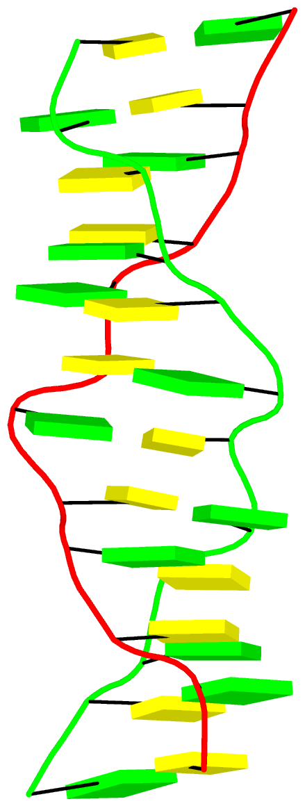
In January 29, 2025, I received the following email request from a long-time DSSR user:
... recently noted that 3DNA/DSSR automatically maps non-standard nucleotides to standard nucleotides. I wonder if you would be willing to share with us your most current version of mappings?
I responded to the user the same day, with detailed information about the mapping process in DSSR. The user was happy with my response, and that thread was quickly closed with a positive note.
On April 22, 2025, a related question, titled "Can x3dna-dssr correctly handle N1-methyl-pseudouridine?", was asked on the 3DNA Forum. In answering the question on the Forum, I referred to my email response to the previous user.
I now realize that writing a detailed blog post explaining the mapping process would be beneficial for DSSR users. It would also enable me to easily reference this blog post in future interactions with users.
3DNA/DSSR performs automatic mapping of modified nucleotides (including pseudouridine) to their standard counterparts. Over the years, the method has proven to work well in real-world applications. It is one of the defining features that make DSSR just work. For example, for the tRNA 1ehz, DSSR automatically identifies the following 14 modified nucleotides (of 11 unique types):
# x3dna-dssr -i=1ehz.pdb
List of 11 types of 14 modified nucleotides
      nt    count  list
   1 1MA-a    1    A.1MA58
   2 2MG-g    1    A.2MG10
   3 5MC-c    2    A.5MC40,A.5MC49
   4 5MU-t    1    A.5MU54
   5 7MG-g    1    A.7MG46
   6 H2U-u    2    A.H2U16,A.H2U17
   7 M2G-g    1    A.M2G26
   8 OMC-c    1    A.OMC32
   9 OMG-g    1    A.OMG34
  10 PSU-P    2    A.PSU39,A.PSU55
  11 YYG-g    1    A.YYG37
Users could run DSSR on a set of structures of interest, and collect the unique mappings for a complete list of modified nucleotides.
Moreover, DSSR has the --nt-mapping option that allows users to control the mapping process. The screenshot below is taken from the relevant part of the DSSR manual.
For example, DSSR automatically maps 5MU (5-methyluridine 5′-monophosphate) to t (i.e., modified thymine) because of the 5-methyl group. With the option --nt-mapping='5MU:u', DSSR would take 5MU as a modified uracil. This option allows for multiple mappings separated by comma. The mapping of 5MU to u or t is obviously arbitrary. DSSR is robust against the ambiguity in designating a modified nucleotide to its nearest canonical counterpart. For example, mapping 5MU to u or t has minimal influence on DSSR-derived base-pair parameters and other structural features.

Background information on the mapping
Over the years, I've refined the heuristics of the mapping process. In the early days with 3DNA, I kept an ever increasing list in file baselist.dat with hundreds of entries like: MIA a that maps MIA as a modified A, denoted as lowercase a. In recent releases of DSSR, I keep only the standard ones, with a total of 48 entries like ADE A, and DG5 G etc. If a residue is not a standard one, the following C function is called to do the mapping. DSSR performs filtering to decide if a residue is a nucleotide, and if so R (purine) or Y (pyrimidine).
static void derive_new_nt_std_name(long resi, struct_mol *pdb, char *info)
{
    char str[BUF512];
    double d1 = DMAX, d2 = DMAX;
    long C1_prime, N1, C5;
    struct_residue *r = &pdb->residues[resi];

    if (r->type[RESIDUE_NT_UNKNOWN]) {
        sprintf(r->std_name, "__%c", Gvars.abasic);
        return;
    }

    if (is_R(resi, pdb)) {  /* purine */
        if (residue_has_atom(" O6 ", resi, pdb))  /* with ' O6 ' */
            strcpy(r->std_name, "__g");
        else if (!residue_has_atom(" N6 ", resi, pdb) &&  /* no ' N6 ' but ' N2 ' */
                 residue_has_atom(" N2 ", resi, pdb))
            strcpy(r->std_name, "__g");
        else
            strcpy(r->std_name, "__a");

    } else {  /* a pyrimidine */
        if (residue_has_atom(" N4 ", resi, pdb))
            strcpy(r->std_name, "__c");
        else if (residue_has_atom(" C7 ", resi, pdb))
            strcpy(r->std_name, "__t");
        else
            strcpy(r->std_name, "__u");

        C1_prime = find_atom_in_residue(" C1'", resi, pdb);
        N1 = find_atom_in_residue(" N1 ", resi, pdb);
        if (atoms_same_model_chain_altloc(C1_prime, N1, pdb))
            d1 = dist_atoms(C1_prime, N1, pdb);

        if (!dval_in_range(d1, 1.0, 2.0)) {
            C5 = find_atom_in_residue(" C5 ", resi, pdb);
            if (atoms_same_model_chain_altloc(C1_prime, C5, pdb))
                d2 = dist_atoms(C1_prime, C5, pdb);
            if (dval_in_range(d2, 1.0, 2.0))
                strcpy(r->std_name, "__p");
        }
    }

    if (!Gvars.standalone) {
        sprintf(str, "\n\tmatched nucleotide '%s' to '%c' for %s\n"
                "\tverify and add an entry in <baselist.dat>\n",
                r->res_name, r->std_name[2], info);
        logit(str);
    }
}
Recently, I read carefully the two papers by Farag et al. on the ASC-G4 algorithm to calculate "advanced structural characteristics of G-quadruplexes" (2023), and the comprehensive analysis results of intramolecular G4 structures in the PDB (2024). By developing a convention to orient and number the four strands, ASC-G4 allows for unambiguous determination of the intramolecular G4 topology. It also has an in-depth discussion on assigning syn or anti glycosidic configuration of guanosines, and categorizes four different types of snapbacks.
I am glad to see that DSSR is cited in these two papers, as quoted below:
X3dna-DSSR (19) (http://x3dna.org) is a website that was created to calculate nucleic acid structural parameters, like the local base-pair parameters, local step base-pair parameters, torsion angles, etc, but not the special characteristics of G4. A subdomain dedicated to G4, DSSR-G4DB (Dissecting the Spatial Structure of RNA – G4 Data Base) (http://g4.x3dna.org) emanated from this website. It is a database that gathers and calculates some specific structural information about published G4s, like the topology, the rise, the helical twist, etc, but not the groove widths or the presence of snapbacks. -- Farag et al. (2023)
Indeed, DSSR-G4DB dose not classify snapbacks. I was aware of such non-canonical G4s when I first developed the G4 module in DSSR around 2017-2018, and the V-shaped loops was derived to reflect the peculiarity of snapbacks.
DSSR classifies groove widths as medium, wide, or narrow, based on the glycosidic angles of neighboring guanosines in a G-tetrad, following the G4 literature. Using PDB entry 2lod as an example, the relevant part of the DSSR output is shown below. The groove widths of the three G-tetrads in the G4-stem have the same pattern of groove=--wn, standing for medium, medium, wide, and narrow, respectively. Note that the medium groove is represented by a dash instead of m because --wn stands out more clearly than mmwn (similar idea applies to glycosidic bond, e.g., sss-).
 1  glyco-bond=sss- sugar=---- groove=--wn Major-->WC N- nts=4 GGGG A.DG1,A.DG6,A.DG20,A.DG16
 2  glyco-bond=---s sugar=---- groove=--wn WC-->Major N+ nts=4 GGGG A.DG2,A.DG7,A.DG21,A.DG15
 3  glyco-bond=---s sugar=---- groove=--wn WC-->Major N+ nts=4 GGGG A.DG3,A.DG8,A.DG22,A.DG14
Since DSSR-G4DB is a database, the user cannot provide his own G4 structure, to obtain structural information. Hence the necessity of developing a website where the user uploads his G4 structure file to obtain all its important and specific structural characteristics (like the topology, the groove width, the tilt and twist angles, etc.). This can be very useful, not only for the analysis of published PDB structures but also for structures in refinement or obtained from MD simulations, to evaluate their quality. To our knowledge, there is no website dedicated to G4 to do such calculations in real-time. Therefore, we developed the algorithm ASC-G4 (advanced structural characteristics of G4) and deployed it as a user-friendly website at the following address: http://tiny.cc/ASC-G4. -- Farag et al. (2023)
Thanks to the NIH R24GM153869 grant support, the http://g4.x3dna.org website now allows users to upload their own atomic structures in PDB for mmCIF format for the identification, annotation, and visualization of G4s. See the example of uploading PDB coordinate file 2lod.pdb.
As background, I had long aspired to develop a dynamic website for on-demand G4 structural analysis but was unable to pursue this goal until recently. During the 4-year funding gap, I still managed to maintain the website g4.x3dna.org, which provides DSSR results for G4 structures in the PDB (a resource now known as the DSSR-G4DB database). To date, the only published work related to G4s is my 2020 paper on the integration of DSSR with PyMOL. Clearly, a dedicated method paper detailing the G4 module in DSSR and the g4.x3dna.org website has been long overdue.
As an initial step toward addressing this gap, I have recently revised the G4-related code in DSSR, fixed existing bugs, and added new features. The g4.x3dna.org website has undergone a complete overhaul, enabling users to upload their own structures for dynamic G4 analysis. Additionally, the DSSR-G4DB database is being actively updated on a weekly basis as new PDB entries are added.
Calculation of the twist and tilt angles. In G4, the helix twist is the rotation of a tetrad relative to its successive one. To measure the twist angle, the most spread method is that described by Lu and Olson (2003) (32) and Reshetnikov et al. (2010) (33). In this method, the angle is calculated from the dot product between two C1’–C1’ vectors from two successive tetrads, i and i + 1, the C1’ atoms of each vector belonging to two adjacent guanosines of a Hbp. The issue with this method is that it does not allow access to the sign of the angle, which defines the direction of the G4 helix, viz. right-handed or left-handed. -- Farag et al. (2023)
There is clearly a misunderstanding in the above text. 3DNA/DSSR can handle left-handed Z-DNA without any issues. DSSR also reports negative twist angles for left-handed G4s, as shown clearly for PDB entry 7d5e, for example.
3DNA/DSSR derives a complete of set of six base-pair parameters (including shear and opening), six step parameters (including twist and rise), and six helical parameters, using a rigorously defined and completely reversible algorithm (CEHS) and the standard base-reference frame. See section "3.2.3 Base pairs" in DSSR User Manual for more details. The DSSR output for G4s (as in DSSR-G4DB) reports only twist and rise, along with overlapped areas, simply because these are the most important parameters and easily interpretable.
The list of the resolved G4 structures was downloaded from the ONQUADRO website (https://onquadro.cs.put.poznan.pl/) (39) at about the end of October 2023. It consisted of 291 intramolecular structures (named unimolecular in the website) and 154 intermolecular G4s (96 bimolecular and 58 tetramolecular). Only the intramolecular structures were kept for this study. To this list, we added 55 missing intramolecular structures that were found on the website of DSSR-G4DB (http://g4.x3dna.org) (40). From the merged list, 345 structures were downloaded from the Protein Data Bank (PDB) (http://www.rscb.org/pdb/) (41) because one structure had no available coordinates in the PDB format (7ZJ5 (42)). -- Farag and Mouawad (2024)
DSSR adopts the frame of reference of Webba da Silva, designating the four strands and grooves of G4-stem as shown below using PDB entries 8ht7 (G1 in syc) and 5ua3 (G1 in anti) as example for the syn or anti glycosidic bond of the 5'-guanosine, respectively.
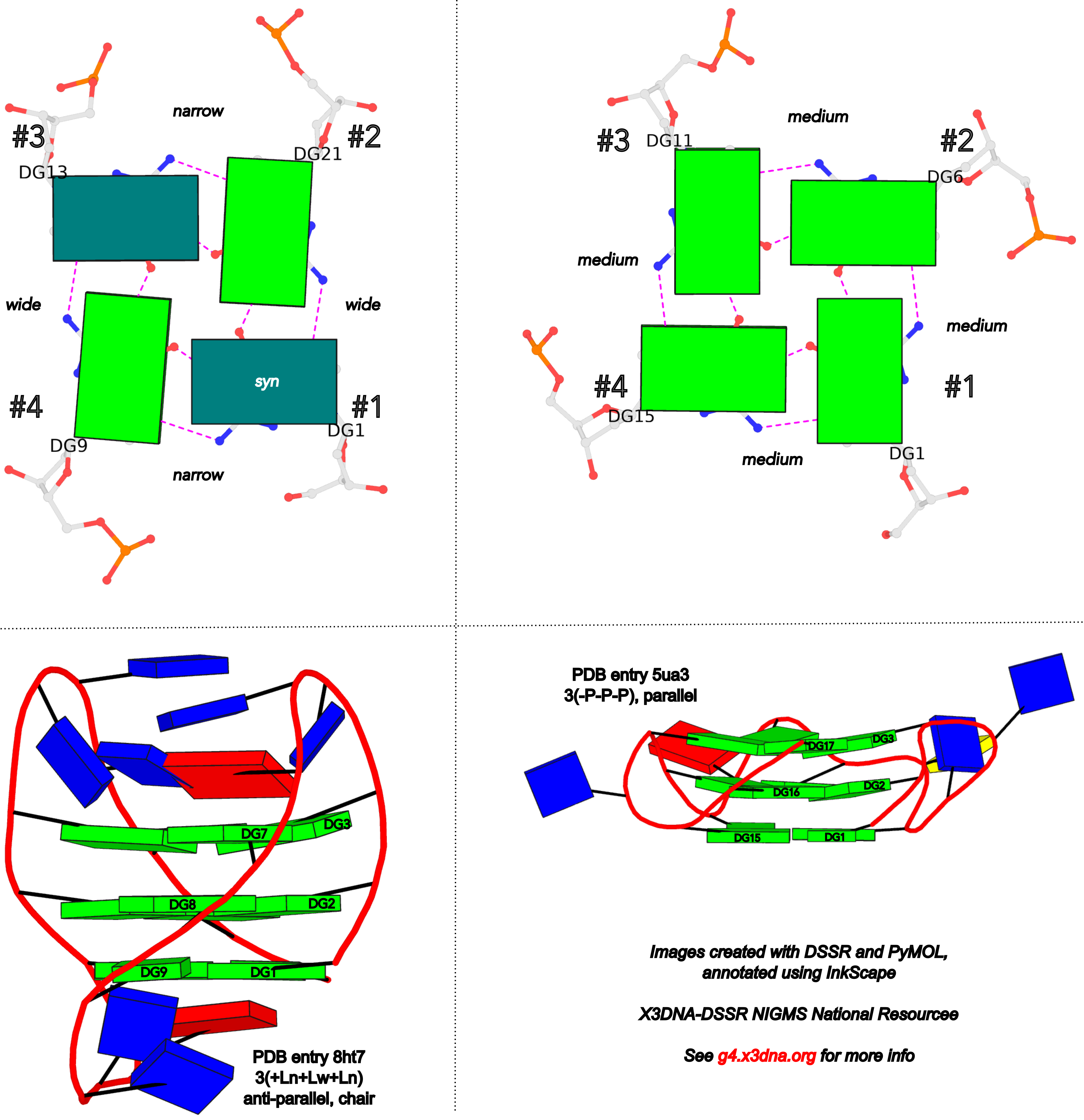
In DSSR, the first strand (#1) is always upward (U) from 5' to 3'-end, and the polarity of the other three strands is determined by its orientation relative to #1: U if parallel, or D if antiparallel. There are a total of 2x2x2=8 possible combinations of U and D for the three strands, which define parallel (U4: UUUU), antiparallel (U2D2: UDDU, UDUD, UUDD), or hybrid (UD3: UDDD; U3D: UDUU, UUDU, UUUD). For example, the PDB entry 2lod is characterized by DSSR as: "hybrid-(mixed), UUUD, U3D(3+1)", and PDB entry 8ht7 as: "anti-parallel, UDUD, chair(2+2)". This notation is topologically equivalent to the one adopted by ASC-G4 but with opposite orientation of the strands.
Overall, DSSR and ASC-G4 provide different perspectives on G4 structures. It is to the user to decide which one is more suitable for their needs.
References
Farag,M. et al. (2023) ASC-G4, an algorithm to calculate advanced structural characteristics of G-quadruplexes. Nucleic Acids Res., 51, 2087–2107.
Farag,M. and Mouawad,L. (2024) Comprehensive analysis of intramolecular G-quadruplex structures: furthering the understanding of their formalism. Nucleic Acids Res., gkae182.
In late September of 2018, I contacted Dr. Mateus Webba da Silva requesting a copy of his 2007 article, titled "Geometric formalism for DNA quadruplex folding". At that time, I had implemented a G4 module within DSSR for the automatic identification, comprehensive annotation, and schematic visualization of G-quadruplexes from 3D atomic coordinates. I noticed the 2007 paper, and was intrigued by the following sentences in the abstract:
A formalism is presented describing the interdependency of a set of structural descriptors as a geometric basis for folding of unimolecular quadruplex topologies. It represents a standard for interpretation of structural characteristics of quadruplexes, and is comprehensive in explicitly harmonizing the results of published literature with a unified language.
Mateus kindly sent me a copy of the 2007 article, and shortly afterwards he also shared with me the Dvorkin et al. (2018) paper on "Encoding canonical DNA quadruplex structure". I carefully read both papers, plus the Karsisiotis et al. (2013) tutorial paper. I was impressed by the elegance of the formalism: simple and systematic, so I immediately decided to add this feature to the G4 module of DSSR.
As the Chinese saying goes, "纸上得来终觉浅,绝知此事要躬行" ("What you learn from books is always shallow. You must practice it yourself to know it well." -- Google Translate). The implementation process was challenging because of subtleties in the formalism, but very rewarding. It is all about scientific understanding and software engineering. Only after a thorough understanding and attention to meticulous details can one create a robust and reliable software tool. On the other hand, once properly implemented, the DSSR G4 module can be applied consistently. Any discrepancies between DSSR output and literature merit further investigation. These discrepancies could either arise from bugs in DSSR (which I will promptly address upon identification) or, more likely, typos or errors in the reported results.
Webba da Silva (2007) systematically described the interdependency of glycosidic bond (syn or anti), strand polarity (parallel or anti-parallel), groove width (narrow, medium, or wide), and loop type (lateral, propeller, or diagonal) in unimolecular G-quadruplexes. Figures 1-3 and Scheme 1 of Webba da Silva (2007) are very informative, and easy to follow conceptually. The Karsisiotis et al. (2013) tutorial provided further details based on experimentally determined G-quadruplex structures from the PDB (e.g., Figure 3: the schematic for all possible combinations of glycosidic bond and the corresponding groove-width combinations in G-tetrad). Some key observations:
- Since glycosidic bond can be either syn or anti, there a total of
2x2x2x2 = 16 possible combinations in a G-tetrad.
- The disposition of glycosidic bond of guanosines in a G-tetrad leads to only eight possible groove-width combinations.
- Only tetrads with the same groove-width combinations may stack to form stable G-quadruplexes.
- Propeller loops invariably link medium grooves within a G-quadruplex stem.
- Lateral and diagonal loops bridge guanosines of different glycosidic bond.
- If a single-stranded quadruplex starts with a narrow groove, it can only be with a clockwise loop progression (i.e., +lateral).
- There are 26 permissible looping combinations within a canonical unimolecular G-quadruplex (G4-stem).
To unambiguously characterize a G4-stem, Webba da Silva (2007) defined a frame of reference where the 5’-G in a G4-stem is set as the origin, and the first strand is progressing towards the viewer. Regardless of the clockwise or anti-clockwise progression of the base sequence, the scheme designates one orientation for the syn and anti glycosidic bond by following G+G H-bonding alignments. Put another way, grooves and strands are strictly related to the reference (first) strand in an anti-clockwise manner, irrespective of the progression of the base sequence. The point is illustrated in the figure below, using PDB entries 8ht7 (G1 in syc) and 5ua3 (G1 in anti) as an example for the syn or anti glycosidic bond of the 5'-guanosine, respectively.
Based on previous work, the Dvorkin et al. (2018) paper proposed a systematic nomenclature for G4-stem. The single structural descriptor contains:
- The number of G-tetrads (i.e., the G-tract length).
- Loop types (lowercase l for lateral, p for propeller, and d for diagonal) and relative direction ("+" for clockwise and "-" for anti-clockwise progression, using the frame of reference described above).
- For lateral loops, the groove widths ("w" for wide, and “n” for narrow) are denoted in subscript.
So a complete descriptor could be 2(+lnd−p), as shown in Figure 1A of the Dvorkin et al. (2018) paper. Significantly, Figure 1B therein further gave structural descriptors for six experimentally determined G4-stems from the PDB. These examples, plus the ones in the supplementary materials, were used to validate my implementation of the systematic nomenclature in the G4 module of DSSR. My results agree with those in the Dvorkin et al. (2018) paper, except for two cases, which are discussed below.
- For PDB entry 2gku: 3(-p-ln-lw) (Dvorkin et al.) vs 3(-P-Lw-Ln) (DSSR), with swapped n (narrow) and w (wide) groove widths for both lateral loops.
- For PDB entry 2lod: 3(-pd+ln) (Dvorkin et al.) vs 3(-PD+Lw) (DSSR), with swapped n (narrow) and w (wide) groove width for the lateral loop.
Note that in DSSR, I am using uppercase L/P/D for lateral/propeller/diagonal loop types, and lowercase n/w for narrow/wide groove widths, respectively. Doing so distinguishes between the different loop types and groove widths in pure text format.
After careful examination of these discrepancies, I still couldn’t find any errors in my implementation. So I contacted Mateus for verification (in early October 2018). Thankfully, he quickly responded and acknowledged the mistakes for PDB entry 2gku in Dvorkin et al. (2018), saying "There can not be a –Ln after the –p." Clearly, the wrong descriptor for PDB entry 2gku in Dvorkin et al. (2018) was due to a typographical error. This example illustrates the power of a robust software tool like DSSR.
References
Dvorkin,S.A. et al. (2018) Encoding canonical DNA quadruplex structure. Sci. Adv., 4, eaat3007.
Karsisiotis,A.I. et al. (2013) DNA quadruplex folding formalism – A tutorial on quadruplex topologies. Methods, 64, 28–35.
Webba da Silva,M. (2007) Geometric formalism for DNA quadruplex folding. Chemistry A European J, 13, 9738–9745.
Over the past few years, the Szachniuk group has made several significant contributions to the field of structural bioinformatics of G-quadruplexes. The following five publications are particularly noteworthy, and I am glad to see that 3DNA/DSSR have been cited in all of them.
1. Zok et al. (2020) -- ElTetrado: a tool for identification and classification of tetrads and quadruplexes
The BMC Bioinformatics paper introduced the ElTetrado software tool for identifying and classifying G-tetrads in unimolecular G-quadruplex structures into ONZ taxonomy. Here DSSR is employed to identify base-pairs and base-stacking interactions.
ElTetrado processes PDB and mmCIF files to identify quadruplexes and their component tetrads in nucleic acid structures (Fig. 2). It applies DSSR [24] to collect the preliminary information about base pairs and stacking.
We recommend that, apart from ElTetrado, the users should download the DSSR binary [24] and place it in the same local directory. DSSR is utilized for the preliminary analysis of base pairs in the input 3D structure. Its local installation allows the users to control DSSR execution. For example, one can decide to pass --symmetry parameter to x3dna-dssr binary when dealing with X-ray structures, which is necessary for some quadruplexes.
As documented in the DSSR Manual, by default, DSSR reads in the first model of an NMR ensemble. A biological unit of X-ray crystal structures in the PDB may contain symmetry-related components formatted as a MODEL/ENDMDL delimited, NMR-like ensemble. In such cases, the --symmetry (or --symm) option is required for DSSR to process the entire biological unit.
For example, x3dna-dssr -i=4ms9.pdb1 --symm leads to the identification of 10 Watson-Crick base pairs in the biological unit of PDB entry 4ms9 (uploaded). The --symm option is now enabled for user-uploaded PDB files on the skmatic.x3dna.org website. Without the --symm option, DSSR would not find any Watson-Crick base pairs in 4ms9.pdb1 since MODEL#1 is single stranded.
Noticing the confusion users may have in using the --symm option, I have revised DSSR to check for overlapped residues. When all models in an NMR ensemble are taken as a whole with the --symm option, there will be overlapped residues. In such cases, DSSR will report a diagnostic message and proceed with the first model only. The final result is as if --symm has not been specified. Put another way, specifying --symm for an NMR ensemble does no harm to the analysis. For example, analyzing PDB entry 8xeq with the --symm option would have the following message and only the first model would be processed.
x3dna-dssr -i=8xeq.pdb --symm -o=8xeq.out
[i] You specified --symm, but the input file is an (NMR) ensemble
    *** in the following, only the FIRST model will be processed ***
Alternatively, if the users do not want to have a local version of DSSR binary, they can obtain the DSSR output in JSON format from any place and use them as input data for ElTetrado (with --dssr-json parameter).
ElTetrado is started from the command line. The users enter the program name and either --pdb followed by an input file name (the file should be in PDB or mmCIF format), or --dssr-json followed by a path to JSON file generated by DSSR, or both switches at once.
The JSON output from DSSR can be obtained directly from the skmatic.x3dna.org website for pre-processed PDB entries or user-supplied coordinate files. For examples, for PDB entry 1ehz, the URL is http://skmatic.x3dna.org/pdb/1ehz/1ehz.json. Alternatively, users can use the web API to get the JSON file, as shown below:
# Pre-processed PDB entry:
curl http://skmatic.x3dna.org/api/pdb/1ehz/json

# With user-supplied PDB file
curl http://skmatic.x3dna.org/api -F 'model=@1ehz.pdb' -F 'type=json'
curl http://skmatic.x3dna.org/api -F 'url=https://files.rcsb.org/download/1ehz.pdb.gz' -F 'type=json'
2. Popenda et al. (2020) -- Topology-based classification of tetrads and quadruplex structures
This paper presents the ONZ scheme to clarify tetrads in unimolecular structures (see Figure 2 therein). Note that DSSR, with option --G4=ONZ, classifies G-tetrads into ONZ taxonomy. For example, the PDB entry 2gku has one G-tetrad (G3, G9, G17, G21) in the O- category, and two G-tetrads in O+.
Structures from both sets were analyzed using self-implemented programs along with DSSR software from the 3DNA suite (Lu et al., 2015). From DSSR, we acquired the information about base pairs and stacking.
3. Zurkowski et al. (2022) -- DrawTetrado to create layer diagrams of G4 structures
DrawTetrado generates static layer diagrams that represent structural data in a pseudo-3D perspective. The layer diagram is very informative and visually pleasing, and it complements the cartoon block schematics generated by the DSSR-PyMOL integration and the detailed DSSR characterization of G-quadruplexes.
So far, the only visual model designed for the 3D structure of quadruplexes is cartoon block schematics (Fig. 1C). These models are generated by DSSR-PyMOL integration and presented as static images of the structure viewed from six perspectives (Lu, 2020).
4. Adamczyk et al. (2023) -- WebTetrado: a webserver to explore quadruplexes in nucleic acid 3D structures
The topologies underlying the classification of quadruplexes and other parameters of their structures can be analyzed using a few computational tools. DSSR (7) was the first to target the detection of G-quadruplexes in 3D structure data saved in PDB and PDBx/mmCIF files and to describe their features. It runs systematically on all entries in the Protein Data Bank and collects motifs found in the DSSR-G4DB database. ElTetrado (8) can identify and analyze G4s and other kinds of tetrads and quadruplexes, classify them, and compute their parameters. It is the core of the computation pipeline running within the ONQUADRO database system (9). The most recent tool for processing atom coordinates in the search for quadruplexes is ASC-G4 (10). It calculates more features than DSSR and ElTetrado, but is limited to unimolecular quadruplexes and supports only the PDB format.
The example illustration in Figure 3 of the paper is on PDB entry 6h1k, the major G-quadruplex form of HIV-1 LTR (long terminal repeat). The layer diagram shown below, re-generated using the WebTetrado website, helps visualize the detailed characterization of DSSR very nicely.
 "In DSSR, a G4-helix is defined by stacking interactions of G-tetrads, regardless of backbone connectivity, and may contain more than one G4-stem." For PDB entry 6h1k, DSSR identifies a G-helix with three G-tetrads, ordered properly. Specifically, strand#1 consists of (G2, G1, and G25), even G1 and G25 are not covalently connected. On the other hand, "In DSSR, a G4-stem is defined as a G4-helix with backbone connectivity. Bulges are also allowed along each of the four strands." Thus, the G4-stem is composed of only two G-tetrads, as detailed below.
Stem#1, 2 G-tetrads, 3 loops, INTRA-molecular, UDDD, hybrid-(mixed), 2(D+PX), UD3(1+3)

 1  glyco-bond=s--- sugar=---- groove=w--n Major-->WC Z- nts=4 GGGG A.DG1,A.DG20,A.DG16,A.DG27
 2  glyco-bond=-sss sugar=.-.3 groove=w--n WC-->Major Z+ nts=4 GGGG A.DG2,A.DG19,A.DG15,A.DG26
  step#1  mm(<>,outward)  area=12.76 rise=3.47 twist=18.2
  strand#1  U DNA glyco-bond=s- sugar=-. nts=2 GG A.DG1,A.DG2
  strand#2  D DNA glyco-bond=-s sugar=-- nts=2 GG A.DG20,A.DG19
  strand#3  D DNA glyco-bond=-s sugar=-. nts=2 GG A.DG16,A.DG15
  strand#4  D DNA glyco-bond=-s sugar=-3 nts=2 GG A.DG27,A.DG26
  loop#1 type=diagonal  strands=[#1,#3] nts=12 GAGGCGTGGCCT A.DG3,A.DA4,A.DG5,A.DG6,A.DC7,A.DG8,A.DT9,A.DG10,A.DG11,A.DC12,A.DC13,A.DT14
  loop#2 type=propeller strands=[#3,#2] nts=2 GC A.DG17,A.DC18
  loop#3 type=diag-prop strands=[#2,#4] nts=5 GACTG A.DG21,A.DA22,A.DC23,A.DT24,A.DG25

List of 2 non-stem G4-loops (including the two closing Gs)
 1 type=lateral   helix=#1 nts=5 GACTG A.DG21,A.DA22,A.DC23,A.DT24,A.DG25
 2 type=V-shaped  helix=#1 nts=4 GGGG A.DG25,A.DG26,A.DG27,A.DG28
DSSR correctly identifies the 12-nt diagonal loop, containing a canonical duplex stem and a hairpin loop. Notably, the G-tetrad (25-21-17-28) does not belong to the G4-stem because of the broken backbone connectivity between G1 and G25. Instead, the Gs in the G-tetrad (25-21-17-28) become part of the following two loops, which are certainly unconventional yet follow naturally the DSSR definition of G4-stem.
- The propeller loop, which now includes G17 (part of the G-tetrad), in addition to C18.
- The unusual diag-prop (diagonal-propeller ) loop, which consists of G21, A22, C23, T24, and G25.
Moreover, DSSR also reports two loops that are not defined by the G4-stem: the V-shaped loop (G25-G26-G27-G28) and the lateral loop (G21-A22-C23-T24-G25). See the notes in the above layer diagram. V-shaped loop occurs when the 5’-endmost G-tetrad lies in the middle of the G-quartets stack as in the non-canonical G4 structures with snapbacks.
The G4-helix and G4-stem definitions parallel those for duplex helix and stem in DSSR. The characterization of loops follows naturally once G4-stem or duplex stem are identified. The unusual propeller and diagonal-propeller loops noted above are due to non-canonical structures, which also lead to the listing of non-stem G4-loops.
I may consider to add special handling of snapbacks (or other worthwhile classes of non-canonical G4 structures) so that the reported loops follow whatever consensus the community agrees upon in the future. Nevertheless, I would like to emphasize that the consistent definitions of G4-stem and loops in DSSR help pinpoint extraordinary features to draw users' attention to non-canonical G4 structures. The layer diagram from DrawTetrado and WebTetrado are very handy in illuminating the basic concept and technical details, as shown here for PDB entry 6h1k.
5. Zok et al. (2022) -- ONQUADRO: a database of experimentally determined quadruplex structures
The computational engine is composed of scripts utilising in-house and third-party procedures, responsible for data collection, quadruplex identification, computation of structure parameters, secondary structure annotation, visualisation of the secondary and tertiary structure models, database queries, generation of statistics, and newsletter preparation. DSSR (--pair-only mode) (36) and ElTetrado (39) functionalities are applied to identify quadruplexes, tetrads, and G4-helices in nucleic acid structures.
References
Adamczyk, B., Zurkowski, M., Szachniuk, M., & Zok, T. (2023). WebTetrado: a webserver to explore quadruplexes in nucleic acid 3D structures. Nucleic Acids Research, 51(W1), W607–W612. https://doi.org/10.1093/nar/gkad346
Popenda, M., Miskiewicz, J., Sarzynska, J., Zok, T., & Szachniuk, M. (2020). Topology-based classification of tetrads and quadruplex structures. Bioinformatics, 36(4), 1129–1134. https://doi.org/10.1093/bioinformatics/btz738
Zok, T., Kraszewska, N., Miskiewicz, J., Pielacinska, P., Zurkowski, M., & Szachniuk, M. (2022). ONQUADRO: a database of experimentally determined quadruplex structures. Nucleic Acids Research, 50(D1), D253–D258. https://doi.org/10.1093/nar/gkab1118
Zok, T., Popenda, M., & Szachniuk, M. (2020). ElTetrado: a tool for identification and classification of tetrads and quadruplexes. BMC Bioinformatics, 21(1), 40. https://doi.org/10.1186/s12859-020-3385-1
Zurkowski, M., Zok, T., & Szachniuk, M. (2022). DrawTetrado to create layer diagrams of G4 structures. Bioinformatics, 38(15), 3835–3836. https://doi.org/10.1093/bioinformatics/btac394
I recently came across the Direk & Doluca (2024) paper on CIIS‐GQ: Computational Identification and Illustrative Standard for representation of unimolecular G‐Quadruplex secondary structures. Since DSSR is mentioned extensively in this work, with a section comparing CIIS-GQ and DSSR in supplementary materials, it is worthwhile to explore the issues raised in the paper. Overall, following literature allows me to clarify misconceptions and fix bugs that further improve DSSR.
The data which contain the G-quadruplexes were identified by DSSR-G4DB website [12, 13, 16]. All of the PDB (protein data bank) ids of DNA and RNA structures are extracted from the aforementioned website and the pdb files which contain the three dimensional data of the corresponding structures were downloaded from the protein data bank [3–5]. [under section "Materials and Methods": "Data"]
The DNA and RNA structures listed in 3DNA website were identified and downloaded from Protein Data Bank. Only unimolecular structures were used for the rest of the study (Supplementary Fig. 2). [under section "Results"]
Additionally, DSSR requires licensing to get annotation results for G-quadruplex structures. Fortunately, the annotation results for a number of G-quadruplexes were already published at DSSR-G4DB (46) and we were able to compare. [under section "Comparison with DSSR" in supplemental materials]
I am glad the DSSR-G4DB website served as a starting point for this study. The G4.x3dna.org website, where DSSR-G4DB is hosted, has always been available to the public. With the NIH R24GM153869 grant support, the standalone DSSR software is free for academic use and can be obtained from the Columbia Technology Ventures (CTV) website.
All obtained results for each pdb file were compared with DSSR. Out of which 35 DNA and 13 RNA structures were analyzed differently (Supplementary Table 2). Significant differences were detected for a number of structures between CIIS-GQ and DSSR analysis. For example, in 1k8p, 3ibk, 6ip7 and 5ccw structures, DSSR fails to identify some loops in some structures.
Most common issue that we have observed with DSSR is that it places loops in wrong places in some structures. For example, In 2a5p structure, the first loop is identified as reversal by both tools but DSSR also assigns the G6 to this loop which already participates in a tetrad. Such misplacement of tetrad-forming guanines in a loop is also seen in other structures such as 2a5r, 2kpr, 2m53, 2m92, etc (Supplementary Table 2).
The G4 module in DSSR was first developed around 2017-2018 and the work was mentioned briefly in the Lu (2020) paper on DSSR-PyMOL integration. However, due to the funding gap, the development of the G4 module was put on hold. I have never got a chance to write a paper documenting the detailed algorithms for the identification, annotation, and visualization of G-quadruplexes. I recently revamped the G4.x3dna.org website from inside out, and reprocessed all PDB structures to compile the DSSR-G4DB database. Along the way, the G4 module has been updated and improved. Now I'm actively working on a manuscript on the G4 module in DSSR and the associate website.
DSSR has clear definitions of G4-helix and G4-stem, and the corresponding loops. Specifically, for PDB entry 2a5p, DSSR reports the following:
## List of 1 G4-helix

In DSSR, a G4-helix is defined by stacking interactions of G-tetrads, regardless of backbone connectivity,
and may contain more than one G4-stem.

##### Helix#1, 3 G-tetrads, INTRA-molecular, with 1 stem

 1  glyco-bond=---- sugar=---- groove=---- WC-->Major O+ nts=4 GGGG A.DG4,A.DG8,A.DG13,A.DG17
 2  glyco-bond=---- sugar=.--- groove=---- WC-->Major O+ nts=4 GGGG A.DG5,A.DG9,A.DG14,A.DG18
 3  glyco-bond=-s-- sugar=-3-- groove=wn-- WC-->Major Z- nts=4 GGGG A.DG6,A.DG24,A.DG15,A.DG19
  step#1  pm(>>,forward)  area=9.64  rise=3.19 twist=32.7
  step#2  pm(>>,forward)  area=12.93 rise=3.29 twist=29.4
  strand#1 DNA glyco-bond=--- sugar=-.- nts=3 GGG A.DG4,A.DG5,A.DG6
  strand#2 DNA glyco-bond=--s sugar=--3 nts=3 GGG A.DG8,A.DG9,A.DG24
  strand#3 DNA glyco-bond=--- sugar=--- nts=3 GGG A.DG13,A.DG14,A.DG15
  strand#4 DNA glyco-bond=--- sugar=--- nts=3 GGG A.DG17,A.DG18,A.DG19
Notice the differences in grooves between the first two G-tetrads vs the 3rd one, and the breaking backbone for strand#2 between G9 and G24.
## List of 1 G4-stem

In DSSR, a G4-stem is defined as a G4-helix with backbone connectivity.
Bulges are also allowed along each of the four strands.

##### Stem#1, 2 G-tetrads, 3 loops, INTRA-molecular, UUUU, parallel, 2(-P-P-P), parallel(4+0)

 1  glyco-bond=---- sugar=---- groove=---- WC-->Major O+ nts=4 GGGG A.DG4,A.DG8,A.DG13,A.DG17
 2  glyco-bond=---- sugar=.--- groove=---- WC-->Major O+ nts=4 GGGG A.DG5,A.DG9,A.DG14,A.DG18
  step#1  pm(>>,forward)  area=9.64  rise=3.19 twist=32.7
  strand#1  U DNA glyco-bond=-- sugar=-. nts=2 GG A.DG4,A.DG5
  strand#2  U DNA glyco-bond=-- sugar=-- nts=2 GG A.DG8,A.DG9
  strand#3  U DNA glyco-bond=-- sugar=-- nts=2 GG A.DG13,A.DG14
  strand#4  U DNA glyco-bond=-- sugar=-- nts=2 GG A.DG17,A.DG18
  loop#1 type=propeller strands=[#1,#2] nts=2 GT A.DG6,A.DT7
  loop#2 type=propeller strands=[#2,#3] nts=3 gGA A.DI10,A.DG11,A.DA12
  loop#3 type=propeller strands=[#3,#4] nts=2 GT A.DG15,A.DT16
Thus the G4-stem consists of two G-tetrads only, and G6 which is part of the 3rd G-tetrad becomes part of a propeller loop. Similar arrangement applies to the other cases.
 DSSR also reports the following loop:
## List of 1 non-stem G4-loop (including the two closing Gs)

 1 type=diagonal  helix=#1 nts=6 GGAAGG A.DG19,A.DG20,A.DA21,A.DA22,A.DG23,A.DG24
In my understanding, the definition and nomenclature of loops in G4 structures are not yet standardized. I am monitoring the development in this field and will update DSSR as needed in due course.
There may also be different types of loops identified by these tools. For example, in 1oz8, which is depicted by CIISGQ as two separate G4s, DSSR fails to identify the G-tetrad, [2, 5, 8, 11], that lies on the outside of the structure. This results in identification of loops formed within this tetrad and its stacking neighbor different to CIIS-GQ. While CIISGQ identifies these loops as reversal, just like the other loops in the structure, DSSR identifies them as non-stem lateral loops. This causes complete misinterpretation of the size and the type of loops in the structure.
The revised DSSR output for PDB entry 1oz8 has the G-tetrad A.DG2,A.DG5,A.DG8,A.DG11 manually added as part of the input, and now all three propeller loops are correctly identified. By default, G11 does not form proper G+G pairs (of LW type cWH or cHW, and Saenger type VI) with G2 and G8. The distortion of the G-tetrad is obvious in the block representation of the structure.
In 4u5m, similar to 1oz8, the structure may be interpreted as two separate G4s connected through a single link (T13,T14). In this case, DSSR identifies only two loops in one of the G4s and labels them as non-stem V-shaped loops. This also differs from CIIS-GQ where CIIS-GQ interprets all loops in both G4 as reversal. Structures containing multiple G4s, such as 1oz8, 4u5m and 6kvb, are often identified with different loop types by DSSR, while CIIS-GQ can recognise the loops correctly and simplifies the comprehension of the structure.
For PDB entry 4u5m, the same arguments above regarding the G4-stem and loops for 2a5p apply.
 1  glyco-bond=s--- sugar=---- groove=w--n Major-->WC O+ nts=4 GGGG A.DG2,A.DG11,A.DG8,A.DG5
 2  glyco-bond=---- sugar=---- groove=---- Major-->WC O+ nts=4 GGGG A.DG3,A.DG12,A.DG9,A.DG6
 3  glyco-bond=---- sugar=---- groove=---- WC-->Major O+ nts=4 GGGG A.DG24,A.DG15,A.DG18,A.DG21
 4  glyco-bond=---- sugar=---- groove=---- WC-->Major O+ nts=4 GGGG A.DG23,A.DG26,A.DG17,A.DG20
As shown, the backbone between G15 and G26 is broken. Moreover, here the assignment of Gs along the strand may need to be manually adjusted.
As shown in Table 1, by relaxing angle and distance parameters, we were able to identify more tetrads (6T2G, 1OZ8) than DSSR, which detects them as multiplets instead.
The current DSSR results for PDB entry 6t2g and 1oz8 are all as expected. Moreover, DSSR can handle PDB entry 6t2g automatically, while for PDB entry 1oz8 user needs to manually edit the input to include the G-tetrad with G11. By allowing users to specify tetrads, DSSR offers precise control and great flexibility, e.g., to include the G-C-G-C tetrads in PDB entry 1a6h.
DSSR has a detailed explanation of strands, tetrads and loops. However, the comprehensive output of DSSR is often hard to understand and grasp the details of the structure. [in supplemental materials]
The detailed explanations are provided to help users understand the DSSR output. They are most insightful in combination with the schematic block diagrams. For examples, for PDB entry 1a6h, the middle G-C-G-C tetrads are crystal clear with the long green and yellow rectangular blocks, specially along with the detailed annotations of the tetrads, as shown below.
 1  glyco-bond=s-s- sugar=---. groove=wnwn Major-->WC -- nts=4 GGGG A.DG1,A.DG11,B.DG8,B.DG4
 2  glyco-bond=---- sugar=-.-- groove=----     --     -- nts=4 CGCG A.DC2,A.DG10,B.DC9,B.DG3
 3  glyco-bond=---- sugar=--.- groove=----     --     -- nts=4 GCGC A.DG3,A.DC9,B.DG10,B.DC2
 4  glyco-bond=-s-s sugar=---- groove=wnwn WC-->Major -- nts=4 GGGG A.DG4,A.DG8,B.DG11,B.DG1
Another advantage of CIIS-GQ is that it requires only two thresholds, the thresholds of distance and angle parameters that can be modified to detect loosely connected tetrads. Due to this advantage, the identification of the tetrads were possible in at least two structures. In case of 1OZ8, DSSR found three tetrads (G1-G4-G7-G10, G13-G16-G19-G22 and G14-G17-G20-G23) as shown at the result page2 (47) while CIIS-GQ has found one more tetrad which is G2-G5-G8-G11. In comparison DSSR highlighted G5-G8-G11 as a multiplet, omitting the G2. Based on this difference, loop classification differs with CIIS-GQ. DSSR has identified 3 stem reversal loops and 3 non-stem lateral loops while we have identified 7 reversal loops. Stem loop is defined as any loop that also forms a duplex within itself.
DSSR now has PDB entry 1oz8 properly characterized, by manually adding the G-tetrad involving G11, as detailed above.
A similar difference exists in 6T2G. DSSR could find 2 tetrads in this structure (G2-G6-G11-G26 and G4-G9-G13-G28) as shown at the result page3 (47) while CIIS-GQ found one more tetrad, G3-G7-G12-G27. DSSR is able to show these four guanines as a multiplet in the list of multiplets section, however does not present it as a tetrad like the other two tetrads. As a result, CIIS-GQ loop types and placements are also different. DSSR has found six lateral loops while CIIS-GQ has found three reversal loops.
DSSR can now handle PDB entry 6t2g automatically. Previous versions of DSSR missed the G-tetrad (G3+G7+G12+G27) because of the G12+G27 pair: it fails the criteria to be classified as the pair of LW type cWH or cHW and Saenger type VI. Thus G3+G7+G12+G27 do not qualify as a G-tetrad, but they still form a multiplet with four guanines.
References
Direk, T., & Doluca, O. (2024). Computational Identification and Illustrative Standard for Representation of Unimolecular G-Quadruplex Secondary Structures (CIIS-GQ). Journal of Computer-Aided Molecular Design, 38(1), 35. https://doi.org/10.1007/s10822-024-00573-1
Lu, X.-J. (2020). DSSR-enabled innovative schematics of 3D nucleic acid structures with PyMOL. Nucleic Acids Research, gkaa426. https://doi.org/10.1093/nar/gkaa426
The legacy PDB format has a field called “altLoc” (alternate location indicator) for "ATOM/HETATM" records in the "Coordinate Section". The corresponding documentation is excerpted below:
COLUMNS        DATA  TYPE    FIELD        DEFINITION
-----------------------------------------------------------------------
17             Character     altLoc       Alternate location indicator.
-
AltLoc is the place holder to indicate alternate conformation. The alternate conformation can be in the entire polymer chain, or several residues or partial residue (several atoms within one residue). If an atom is provided in more than one position, then a non-blank alternate location indicator must be used for each of the atomic positions. Within a residue, all atoms that are associated with each other in a given conformation are assigned the same alternate position indicator. There are two ways of representing alternate conformation- either at atom level or at residue level (see examples).
- For atoms that are in alternate sites indicated by the alternate site indicator, sorting of atoms in the ATOM/HETATM list uses the following general rules:
- In the simple case that involves a few atoms or a few residues with alternate sites, the coordinates occur one after the other in the entry.
- In the case of a large heterogen groups which are disordered, the atoms for each conformer are listed together.
In mmCIF format, AltLoc is under the atom_site category, with attribute name label_alt_id: i.e., labelled as _atom_site.label_alt_id. It is a required data item and appears in 43% of entries in the PDB.
In 3DNA and DSSR, AltLoc has a default value of "A1 ": an atom is taken into consideration if its AltLoc field (a single character) is space, A, or 1, otherwise it is ignored. Note that for mmCIF format, AltLoc field with dot (.) or question mark (?) is taken as space. Customized AltLoc values can be set via the --altloc option in DSSR.
Here is an example. PDB entry 7o1h is a 31-mer synthetic construct, with a hybrid-2R quadruplex-duplex of 3(-P-P-Lw) topology and three syn guanosines. It contains two modified residues designated BGM (BGM26 and BGM28), 8-bromo-2'-deoxyguanosine-5'-monophosphate, with AltLoc set to B. By default, DSSR detects only one G-tetrad, consisting of DG5,DG9,DG13,DG27, ignoring the two G-tetrads with BGM26 and BGM28. With the --altloc=B option (space is always included), all three G-tetrads are detected and the G-quadruplex (a G4-stem) is then automatically annotated as 3(-P-P-Lw):
# x3dna-dssr -i=7o1h-assembly1.cif --altloc=B

List of 2 types of 3 modified nucleotides
      nt    count  list
   1 BGM-g    2    A.BGM26,A.BGM28
   2 THM-t    1    A.THM1

List of 1 G4-stem
  Note: a G4-stem is defined as a G4-helix with backbone connectivity.
        Bulges are also allowed along each of the four strands.
  stem#1[#1] layers=3 INTRA-molecular loops=3 descriptor=3(-P-P-Lw) note=hybrid-2R(3+1) UUUD hybrid-(mixed)
   1  glyco-bond=---s sugar=---. groove=--wn WC-->Major nts=4 GGGg A.DG4,A.DG8,A.DG12,A.BGM28
   2  glyco-bond=---s sugar=--.- groove=--wn WC-->Major nts=4 GGGG A.DG5,A.DG9,A.DG13,A.DG27
   3  glyco-bond=---s sugar=---- groove=--wn WC-->Major nts=4 GGGg A.DG6,A.DG10,A.DG14,A.BGM26
    step#1  pm(>>,forward)  area=13.57 rise=3.39 twist=26.7
    step#2  pm(>>,forward)  area=12.00 rise=3.44 twist=28.4
    strand#1  U DNA glyco-bond=--- sugar=--- nts=3 GGG A.DG4,A.DG5,A.DG6
    strand#2  U DNA glyco-bond=--- sugar=--- nts=3 GGG A.DG8,A.DG9,A.DG10
    strand#3  U DNA glyco-bond=--- sugar=-.- nts=3 GGG A.DG12,A.DG13,A.DG14
    strand#4  D DNA glyco-bond=sss sugar=.-- nts=3 gGg A.BGM28,A.DG27,A.BGM26
    loop#1 type=propeller strands=[#1,#2] nts=1 T A.DT7
    loop#2 type=propeller strands=[#2,#3] nts=1 T A.DT11
    loop#3 type=lateral   strands=[#3,#4] nts=11 ACGCGCAGCGT A.DA15,A.DC16,A.DG17,A.DC18,A.DG19,A.DC20,A.DA21,A.DG22,A.DC23,A.DG24,A.DT25
See G4.x3dna.org for DSSR-enabled annotation and visualization of this G4 structure. Here is the G4-stem in the frame of reference of 5' DG4 (bottom right), following the convention of Dvorkin et al. (2018). It is orientated automatically based on the standard base-reference frame (Olson et al. (2001)) of DG4.
References:
- Dvorkin, Scarlett A., Andreas I. Karsisiotis, and Mateus Webba Da Silva. 2018. “Encoding Canonical DNA Quadruplex Structure.” Science Advances 4 (8): eaat3007. https://doi.org/10.1126/sciadv.aat3007.
- Olson, Wilma K, Manju Bansal, Stephen K Burley, Richard E Dickerson, Mark Gerstein, Stephen C Harvey, Udo Heinemann, et al. 2001. “A Standard Reference Frame for the Description of Nucleic Acid Base-Pair Geometry.” Journal of Molecular Biology 313 (1): 229–37. https://doi.org/10.1006/jmbi.2001.4987.
DNA and RNA are biological macromolecules consisting of long chains of nucleotides. In PDB coordinate files, each DNA/RNA chain is assigned a unique identifier. For the legacy PDB format, the size of the chain identifier is clearly defined to be one alphanumeric character. For the mmCIF format, the length of the chain identifier is flexible: it is normally up to 4-char long, but assembly files can have chain identifiers longer than 4 characters (as of May 2022, see examples).
Recently, I was approached with the following bug report where DSSR v2.4-2021nov11 was used:
Processing file '8feo-assembly1.cif'

[i] '8feo-assembly1.cif' taken as in .cif format by file extension.

*** buffer overflow detected ***: terminated

Aborted
I ran a newer version of DSSR (including the current release v2.5.2-2025apr03) on 8feo-assembly1.cif without any issue, as shown below:
# x3dna-dssr -i=8feo-assembly1.cif -o=8feo.out
[i] '8feo-assembly1.cif' taken as in .cif format by file extension.

Processing file '8feo-assembly1.cif'
[w] chain id 'AAA-2' > 4 chars
...

# Excerpt from 8feo.out
    no. of DNA/RNA chains: 2 [AAA=16,AAA-2=16]
    no. of nucleotides:    32
...
List of 16 base pairs
     nt1            nt2            bp  name        Saenger   LW   DSSR
   1 AAA.A1         AAA-2.U16      A-U WC          20-XX     cWW  cW-W
   2 AAA.G2         AAA-2.C15      G-C WC          19-XIX    cWW  cW-W
   3 AAA.A3         AAA-2.U14      A-U WC          20-XX     cWW  cW-W
The message [w] chain id 'AAA-2' > 4 chars is saying that the chain identifier ‘AAA-2’ is out of the 4-char limit.
In addition to 8feo, similar issues were also fixed for related PDB entries 5a79, 6a7a, 8feo, 8fep, 8feq, 7umk, and 4v3p. Note that 4v3p is a eukaryotic polyribosomal assembly which takes several hours to run on a MacBookPro with 32GB RAM.
Some background information on how DSSR handles chain identifiers for mmCIF format files
When mmCIF support was first added to DSSR in 2013, I hard-coded the chain identifier to 4 chars following the documentation. In early 2024, when running DSSR on weekly updated PDB entries, I noticed a core dump bug with PDB entry 8feo for its biological assembly 1. At that time, I was not aware of the update on mmCIF-Formatted Assembly Files and its expansion of chain identifiers for symmetry-related copies: with PDB assembly files, -# is appended to any chain that is generated by a symmetry operation. So if the base chain id has 3 chars (e.g., AAA), the symmetry related chain will have 5 chars (e.g., AAA-2).
That is the case for PDB entry 8feo: it has a chain with identifier AAA-2 which is symmetry-related to the asymmetric unit chain AAA. Since AAA-2 (5-char long) is above the hard-coded 4-char limit, DSSR crashed (out of array boundary in C). After recognizing the issue, I've increased the chain identifier limit in DSSR to 8 chars, more than enough for all current PDB entries. Moreover, DSSR performs sanity check of chain identifier length: it reports diagnostic message as shown above for chains with over 4-char identifiers (e.g., AAA-2), and automatically shortens long chains to the enlarged limit. DSSR is now more robust and user friendly: it no longer simply crashes, but communicates helpful info about unusual cases to draw users' attention.
Taking this opportunity, I have also proactively updated DSSR to support long atom names , residue names, and segment ids, in preparation for future id changes. Tracing issues to their root causes and fixing them systematically is a key part that makes DSSR a reliable tool for structural bioinformatics. Tests have been added to the quality control infrastructure to ensure that all these new features work as expected.
Nowadays, the vast majority (over 90%) of users’ questions about DSSR can be answered straight away simply because they have already been addressed in advance, as shown in the above example for long chain identifiers. I'm always on the lookout for issues reported on the 3DNA Forum, received from email, Zoom, or in person, and more systematically via DSSR update on weekly released PDB entries, and uploaded files on the web-services (g4.x3dna.org and skmatic.x3dna.org). Every issue is an opportunity to further polish DSSR and make it better. Overall, users’ feedback is invaluable to me: I take it as an asset instead of a burden.
Documentation on chain identifiers in PDB and mmCIF formats
PDB format
The Coordinate Section in the PDB format documentation contains the following for ATOM/HETATM records:
The ATOM records present the atomic coordinates for standard amino acids and nucleotides. ... Non-polymer chemical coordinates use the HETATM record type.
Record Format
COLUMNS        DATA  TYPE    FIELD        DEFINITION
-----------------------------------------------------------
22             Character     chainID      Chain identifier.
**Details**
- Non-blank alphanumerical character is used for chain identifier.
So the chain identifier in PDB format is a single alphanumeric character in column 22 of the ATOM/HETATM records.
mmCIF format
-
Large Structures Represented in mmCIF/PDBx:
Chain identifiers of up to 4 characters are permitted. The PDB chain identifier corresponds to the "_atom_site.auth_asym_id" data item.
-
News item on Distributing PDBx/mmCIF-Formatted Assembly Files
- Github repo on Sample assembly files in PDBx/mmCIF Format
These updated PDBx/mmCIF format assembly files files will include all symmetry generated copies of each chain within a single model, with distinct chain IDs assigned to each. Generation of distinct chain IDs in assembly files are based upon the following rules:
- Chain IDs of the original chains from the atomic coordinate file will be retained (e.g., A)
- Assign unique chain ID for each symmetry copy within a single model. Rules of chain ID assignments:
- The applied index of the symmetry operator will be appended to the original chain ID separated by a dash (e.g., A-2, A-3, etc.)
- If there are more than one type of symmetry operators applied to generate symmetry copy, a dash sign will be used between two operators (e.g., A-12-60, A-60-88, etc.)
Recently, I came across the paper by Mitra et al. (2025) titled "RNAproDB: A Webserver and Interactive Database for Analyzing Protein-RNA Interactions." I am glad to notice that DSSR (Lu et al. 2015) has been cited extensively in this work, as follows:
As part of the processing pipeline, multiple software is run including DSSR^12^ (base-pairing geometries, protein–RNA hydrogen bonds, and RNA secondary structure), HBPLUS^17^ (hydrogen bonds involving water molecules), ... Leontis-Westhof^27^ base pair annotations (as computed by DSSR^12^) ... The structural elements (stems, loops, hairpins, junctions, etc.) are detected using DSSR^12^ and mapped to the partial projection layout (via averaging corresponding residue coordinates)... We explored the relative abundance of different standard nucleotides (A, C, G, and U) in helical vs. non-helical regions (as computed by DSSR^12^)...We quantified the propensity of base-pairing (as detected by DSSR^12^) between different RNA bases (Fig. 3D).
This is an impressive contribution on the characterization of protein-RNA interactions. Reading carefully through the paper and its supplemental PDF, I was intrigued by the following note on a water-mediated U-U base pair missed by DSSR.
Another important aspect to discuss is RNA–RNA water-mediated interactions^33,34^. ... One such example is the CUG repeat structure from PDB ID 7Y2B^35^ (Fig. S5A). The U/U mismatches in this structure are often unable to form direct hydrogen bonds (specifically, the central U/U mismatch forms no direct hydrogen bond). Therefore, DSSR^12^ does not classify it as a base pair. However, two water molecules form water-mediated hydrogen bonds between the two U bases. ...
While DSSR internally already takes consideration of water-mediated H-bonds in the detection of base pairs, it still requires: (1) at least one direct H-bond between two base atoms or a base atom to backbone, and (2) a co-planar geometry between the two bases. The water-mediated U7-U7 pair in PDB entry 7Y2B does not fulfill condition (1): the minimal distance between the two U bases is 5 Å, which is far larger than a typical H-bonding distance. Therefore, DSSR did not classify it as a base pair.
Prompted by the observation of Mitra et al. (2025), I have added a new option (--pair-water) in the DSSR v2.5.1-2025mar19 release to allow for water-mediated base pairs to be detected. Using PDB entry 7Y2B as an example, the DSSR command and related base-pairs output are shown below.
# x3dna-dssr -i=7Y2B.pdb1 --symm --pair-water

List of 13 base pairs
     nt1            nt2            bp  name        Saenger   LW   DSSR
   1 1:S.U1         2:S.A13        U-A WC          20-XX     cWW  cW-W
   2 1:S.U2         2:S.A12        U-A WC          20-XX     cWW  cW-W
   3 1:S.C3         2:S.G11        C-G WC          19-XIX    cWW  cW-W
   4 1:S.U4         2:S.U10        U-U --          --        cWW  cW-W
   5 1:S.G5         2:S.C9         G-C WC          19-XIX    cWW  cW-W
   6 1:S.C6         2:S.G8         C-G WC          19-XIX    cWW  cW-W
   7 1:S.U7         2:S.U7         U-U Water       --        cWW  cW-W
   8 1:S.G8         2:S.C6         G-C WC          19-XIX    cWW  cW-W
   9 1:S.C9         2:S.G5         C-G WC          19-XIX    cWW  cW-W
  10 1:S.U10        2:S.U4         U-U --          --        cWW  cW-W
  11 1:S.G11        2:S.C3         G-C WC          19-XIX    cWW  cW-W
  12 1:S.A12        2:S.U2         A-U WC          20-XX     cWW  cW-W
  13 1:S.A13        2:S.U1         A-U WC          20-XX     cWW  cW-W
Base pair #7 is water-mediated, as shown in the molecular image below. Note that .pdb1 means biological unit 1, and the option --symm reads the two symmetry-related structures in the MODEL/ENDMDL delineated ensemble as a single structure. See the DSSR User Manual for more details.
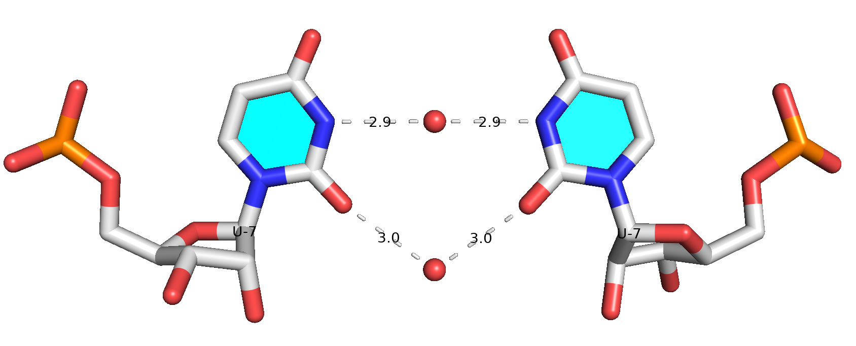
References
-
Lu, Xiang-Jun, Harmen J. Bussemaker, and Wilma K. Olson. 2015. “DSSR: An Integrated Software Tool for Dissecting the Spatial Structure of RNA.” Nucleic Acids Research, July, gkv716. https://doi.org/10.1093/nar/gkv716.
- Mitra, Raktim, Ari S. Cohen, Wei Yu Tang, Hirad Hosseini, Yongchan Hong, Helen M. Berman, and Remo Rohs. 2025. “RNAproDB: A Webserver and Interactive Database for Analyzing Protein-RNA Interactions.” Journal of Molecular Biology, February, 169012. https://doi.org/10.1016/j.jmb.2025.169012.
Cover images provided by X3DNA-DSSR, an NIGMS National Resource for structural bioinformatics of nucleic acids (R24GM153869; skmatics.x3dna.org). Image generated using DSSR and PyMOL (Lu XJ. 2020. Nucleic Acids Res 48: e74).
See the 2020 paper titled "DSSR-enabled innovative schematics of 3D nucleic acid structures with PyMOL" in Nucleic Acids Research and the corresponding Supplemental PDF for details. Many thanks to Drs. Wilma Olson and Cathy Lawson for their help in the preparation of the illustrations.
Details on how to reproduce the cover images are available on the 3DNA Forum.

Structure of the human minor spliceosome pre-B complex (PDB id: 8Y7E; Bai R, Yuan M, Zhang P, Luo T, Shi Y, Wan R. 2024. Structural basis of U12-type intron engagement by the fully assembled human minor spliceosome. Science 383: 1245–1252). The protein–RNA assembly reveals the mechanisms of recognition and recruitment of several small nuclear ribonucleoproteins (snRNPs) involved in the splicing of U12-type introns. The pre-mRNA is depicted by a red ribbon, and the U12 small nuclear RNA (snRNA) by a green ribbon, with bases and Watson-Crick base pairs represented as color-coded blocks: A/A-U in red, C/C-G in yellow, G/G-C in green, U/U-A in cyan; the proteins are shown as gold ribbons. Cover image provided by X3DNA-DSSR, an NIGMS National Resource for structural bioinformatics of nucleic acids (R24GM153869; skmatics.x3dna.org). Image generated using DSSR and PyMOL (Lu XJ. 2020. Nucleic Acids Res 48: e74).

Human tRNA splicing endonuclease (TSEN) complex bound to pre-tRNAArg (PDB id: 7UXA; Hayne CK, Butay KJ, Stewart ZD, Krahn JM, Perera L, Williams JG, Petrovitch RM, Deterding LJ, Matera AG, Borgnia MJ, Stanley RE. 2023. Structural basis for pre-tRNA recognition and processing by the human tRNA splicing endonuclease complex. Nat Struct Mol Biol 30: 824–833). Cryo-EM structure of the TSEN protein assembly with pre-tRNAArg provides insights into the recognition and splicing of an intron that must be removed from the pre-tRNA before translation. The pre-tRNAArg is depicted by a red ribbon, with bases and Watson-Crick base pairs represented as color-coded blocks: A/A-U in red, C/C-G in yellow, G/G-C in green, U/U-A in cyan; the TSEN subunits are shown as gold ribbons. Cover image provided by X3DNA-DSSR, an NIGMS National Resource for structural bioinformatics of nucleic acids (R24GM153869; skmatics.x3dna.org). Image generated using DSSR and PyMOL (Lu XJ. 2020. Nucleic Acids Res 48: e74).

Systemic RNA interference defective protein 1 (SID1) in complex with dsRNA (PDB id: 8XC1; Wang R, Cong Y, Qian D, Yan C, Gong D. 2024. Structural basis for double-stranded RNA recognition by SID1. Nucleic Acids Res 52: 6718–6727). The cryo-EM structure provides a major step towards understanding the mechanism of dsRNA recognition by SID1, involving extensive interactions between basic amino-acid residues and the sugar-phosphate backbone. The dsRNA chains are depicted by red, green, blue, and yellow ribbons, with bases and Watson-Crick base pairs represented as color-coded blocks and minor-groove edges colored white: A/A-U in red, C/C-G in yellow, G/G-C in green, U/U-A in cyan; SID1 is shown by a gold ribbon. Cover image provided by X3DNA-DSSR, an NIGMS National Resource for structural bioinformatics of nucleic acids (R24GM153869; skmatics.x3dna.org). Image generated using DSSR and PyMOL (Lu XJ. 2020. Nucleic Acids Res 48: e74).

Complex of arginyl-tRNA-protein transferase 1 (ATE1) with tRNAArg and a short peptide substrate (PDB id: 8UAU; Lan X, Huang W, Kim SB, Fu D, Abeywansha T, Lou J, Balamurugan U, Kwon YT, Ji CH, Taylor DJ, Zhang Y. 2024. Oligomerization and a distinct tRNA-binding loop are important regulators of human arginyl-transferase function. Nat Commun 15: 6350). The ATE1 homodimer dissociates upon binding the peptide and forms a loop that wraps around tRNAArg. The tRNAArg is depicted by a red ribbon, with bases and Watson–Crick base pairs represented as color-coded blocks: A/A-U in red, C/C-G in yellow, G/G-C in green, U/U-A in cyan; ATE1 is shown by a gold ribbon and the peptide by a white ribbon. Cover image provided by X3DNA-DSSR, an NIGMS National Resource for structural bioinformatics of nucleic acids (R24GM153869; skmatics.x3dna.org). Image generated using DSSR and PyMOL (Lu XJ. 2020. Nucleic Acids Res 48: e74).

Structure of endoribonuclease P (RNase P) in complex with pre-tRNAHis-Ser (PDB id: 8CBK; Meynier V, Hardwick SW, Catala M, Roske JJ, Oerum S, Chirgadze DY, Barraud P, Yue WW, Luisi BF, Tisné C. 2024. Structural basis for human mitochondrial tRNA maturation. Nat Commun 15: 4683). The structure reveals the first step of human mitochondrial tRNA maturation by RNase P, processing the 5′-leader of pre-tRNA. The RNA is depicted by a red ribbon, with bases and Watson-Crick base pairs represented as color-coded blocks: A/A-U in red, C/C-G in yellow, G/G-C in green, U/U-A in cyan; the protein assembly is shown by the gold ribbons. Cover image provided by X3DNA-DSSR, an NIGMS National Resource for structural bioinformatics of nucleic acids (R24GM153869; skmatics.x3dna.org). Image generated using DSSR and PyMOL (Lu XJ. 2020. Nucleic Acids Res 48: e74).

Structure of a group II intron ribonucleoprotein in the pre-ligation state (PDB id: 8T2R; Xu L, Liu T, Chung K, Pyle AM. 2023. Structural insights into intron catalysis and dynamics during splicing. Nature 624: 682–688). The pre-ligation complex of the Agathobacter rectalis group II intron reverse transcriptase/maturase with intron and 5′-exon RNAs makes it possible to construct a picture of the splicing active site. The intron is depicted by a green ribbon, with bases and Watson-Crick base pairs represented as color-coded blocks: A/A-U in red, C/C-G in yellow, G/G-C in green, U/U-A in cyan; the 5′-exon is shown by white spheres and the protein by a gold ribbon. Cover image provided by X3DNA-DSSR, an NIGMS National Resource for structural bioinformatics of nucleic acids (R24GM153869; skmatics.x3dna.org). Image generated using DSSR and PyMOL (Lu XJ. 2020. Nucleic Acids Res 48: e74).

Complex of terminal uridylyltransferase 7 (TUT7) with pre-miRNA and Lin28A (PDB id: 8OPT; Yi G, Ye M, Carrique L, El-Sagheer A, Brown T, Norbury CJ, Zhang P, Gilbert RJ. 2024. Structural basis for activity switching in polymerases determining the fate of let-7 pre-miRNAs. Nat Struct Mol Biol 31: 1426–1438). The RNA-binding pluripotency factor LIN28A invades and melts the RNA and affects the mechanism of action of the TUT7 enzyme. The RNA backbone is depicted by a red ribbon, with bases and Watson-Crick base pairs represented as color-coded blocks: A/A-U in red, C/C-G in yellow, G/G-C in green, U/U-A in cyan; TUT7 is represented by a gold ribbon and LIN28A by a white ribbon. Cover image provided by X3DNA-DSSR, an NIGMS National Resource for structural bioinformatics of nucleic acids (R24GM153869; skmatics.x3dna.org). Image generated using DSSR and PyMOL (Lu XJ. 2020. Nucleic Acids Res 48: e74).

Cryo-EM structure of the pre-B complex (PDB id: 8QP8; Zhang Z, Kumar V, Dybkov O, Will CL, Zhong J, Ludwig SE, Urlaub H, Kastner B, Stark H, Lührmann R. 2024. Structural insights into the cross-exon to cross-intron spliceosome switch. Nature 630: 1012–1019). The pre-B complex is thought to be critical in the regulation of splicing reactions. Its structure suggests how the cross-exon and cross-intron spliceosome assembly pathways converge. The U4, U5, and U6 snRNA backbones are depicted respectively by blue, green, and red ribbons, with bases and Watson-Crick base pairs shown as color-coded blocks: A/A-U in red, C/C-G in yellow, G/G-C in green, U/U-A in cyan; the proteins are represented by gold ribbons. Cover image provided by X3DNA-DSSR, an NIGMS National Resource for structural bioinformatics of nucleic acids (R24GM153869; skmatics.x3dna.org). Image generated using DSSR and PyMOL (Lu XJ. 2020. Nucleic Acids Res 48: e74).

Structure of the Hendra henipavirus (HeV) nucleoprotein (N) protein-RNA double-ring assembly (PDB id: 8C4H; Passchier TC, White JB, Maskell DP, Byrne MJ, Ranson NA, Edwards TA, Barr JN. 2024. The cryoEM structure of the Hendra henipavirus nucleoprotein reveals insights into paramyxoviral nucleocapsid architectures. Sci Rep 14: 14099). The HeV N protein adopts a bi-lobed fold, where the N- and C-terminal globular domains are bisected by an RNA binding cleft. Neighboring N proteins assemble laterally and completely encapsidate the viral genomic and antigenomic RNAs. The two RNAs are depicted by green and red ribbons. The U bases of the poly(U) model are shown as cyan blocks. Proteins are represented as semitransparent gold ribbons. Cover image provided by X3DNA-DSSR, an NIGMS National Resource for structural bioinformatics of nucleic acids (R24GM153869; skmatics.x3dna.org). Image generated using DSSR and PyMOL (Lu XJ. 2020. Nucleic Acids Res 48: e74).

Structure of the helicase and C-terminal domains of Dicer-related helicase-1 (DRH-1) bound to dsRNA (PDB id: 8T5S; Consalvo CD, Aderounmu AM, Donelick HM, Aruscavage PJ, Eckert DM, Shen PS, Bass BL. 2024. Caenorhabditis elegans Dicer acts with the RIG-I-like helicase DRH-1 and RDE-4 to cleave dsRNA. eLife 13: RP93979. Cryo-EM structures of Dicer-1 in complex with DRH-1, RNAi deficient-4 (RDE-4), and dsRNA provide mechanistic insights into how these three proteins cooperate in antiviral defense. The dsRNA backbone is depicted by green and red ribbons. The U-A pairs of the poly(A)·poly(U) model are shown as long rectangular cyan blocks, with minor-groove edges colored white. The ADP ligand is represented by a red block and the protein by a gold ribbon. Cover image provided by X3DNA-DSSR, an NIGMS National Resource for structural bioinformatics of nucleic acids (R24GM153869; skmatics.x3dna.org). Image generated using DSSR and PyMOL (Lu XJ. 2020. Nucleic Acids Res 48: e74).
Moreover, the following 30 [12(2021) + 12(2022) + 6(2023)] cover images of the RNA Journal were generated by the NAKB (nakb.org).
Cover image provided by the Nucleic Acid Database (NDB)/Nucleic Acid Knowledgebase (NAKB; nakb.org). Image generated using DSSR and PyMOL (Lu XJ. 2020. Nucleic Acids Res 48: e74).
DSSR produces RNA secondary structures in connect table (.ct) format. According to "RNAstructure Command Line Help: File Formats" (with slight editing):
CT File Format
A CT (Connectivity Table) file contains secondary structure information for a sequence. These files are saved with a CT extension. When entering a structure to calculate the free energy, the following format must be followed.
- Start of first line: number of bases in the sequence
- End of first line: title of the structure
- Each of the following lines provides information about a given base in the sequence. Each base has its own line, with these elements in order:
- Base number: index n
- Base (A, C, G, T, U, X)
- Index n-1
- Index n+1
- Number of the base to which n is paired. No pairing is indicated by 0 (zero).
- Natural numbering. RNAstructure ignores the actual value given in natural numbering, so it is easiest to repeat n here.
Using PDB entry 1msy as an example (see Figure 1 below):
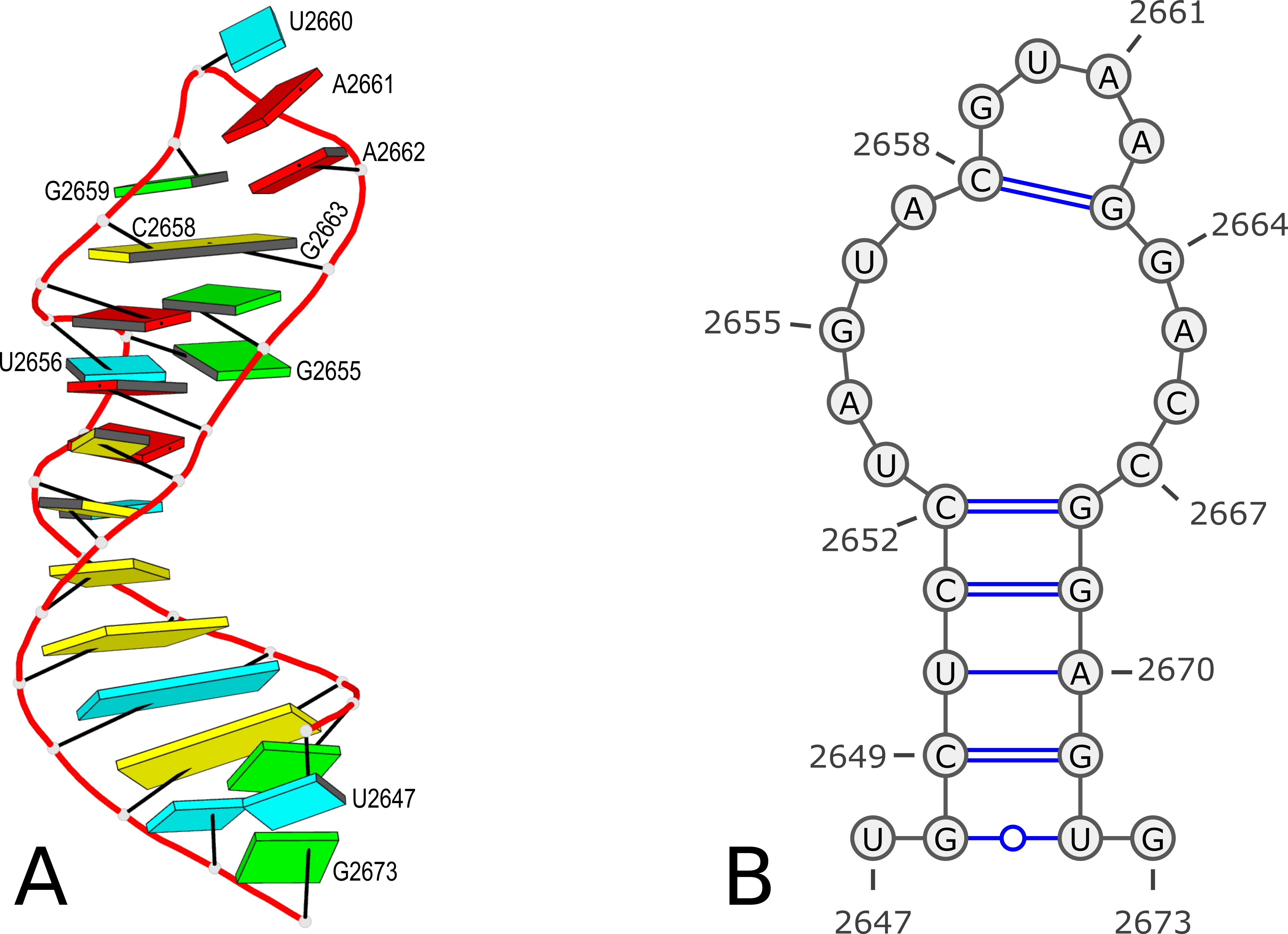
Figure 1. 3D and 2D structures of PDB entry 1msy. (A) 3D schematic auto-created via the DSSR-PyMOL integration. The labeled residues follow PDB coordinates. (B) 2D diagram rendered with VARNA using DSSR-derived 2D structural information in the .ct format. This figure was annotated using Inkscape.
With commands:
x3dna-dssr -i=1msy.pdb
cp dssr-2ndstrs.ct 1msy-dssr-default.ct
The file 1msy-dssr-default.ct has the following contents:
   27 ENERGY = 0.0 [1msy] -- secondary structure derived by DSSR
    1 U     0     2     0  2647
    2 G     1     3    26  2648
    3 C     2     4    25  2649
    4 U     3     5    24  2650
    5 C     4     6    23  2651
    6 C     5     7    22  2652
    7 U     6     8     0  2653
    8 A     7     9     0  2654
    9 G     8    10     0  2655
   10 U     9    11     0  2656
   11 A    10    12     0  2657
   12 C    11    13    17  2658
   13 G    12    14     0  2659
   14 U    13    15     0  2660
   15 A    14    16     0  2661
   16 A    15    17     0  2662
   17 G    16    18    12  2663
   18 G    17    19     0  2664
   19 A    18    20     0  2665
   20 C    19    21     0  2666
   21 C    20    22     0  2667
   22 G    21    23     6  2668
   23 G    22    24     5  2669
   24 A    23    25     4  2670
   25 G    24    26     3  2671
   26 U    25    27     2  2672
   27 G    26     0     0  2673
Here the first line contains 27 (as the number of bases) and ENERGY = 0.0 [1msy] -- secondary structure derived by DSSR (as the title). While RNAstructure ignores the actual values given in natural numbering, DSSR outputs the residue numbers of the nucleotides (e.g. U2467 and G2673) in the PDB file.
With the DSSR option --structure-title (or --str-title, actually via regex "^-?-?str(ucture)?[-_]?title"), users can set the title for the derived .ct file, as shown below:
x3dna-dssr -I=1msy.pdb --structure-title='CT file derived from DSSR'
cp dssr-2ndstrs.ct 1msy-dssr-title.ct

   27 CT file derived from DSSR
    1 U     0     2     0  2647
    2 G     1     3    26  2648
......
   26 U    25    27     2  2672
   27 G    26     0     0  2673
One can also remove the title, by using an empty string "" (i.e., --str-title="") or simply --str-title (or --str-title=).
x3dna-dssr -I=1msy.pdb --structure-title=""
cp dssr-2ndstrs.ct 1msy-dssr-notitle.ct

   27
    1 U     0     2     0  2647
    2 G     1     3    26  2648
......
With the --more option, DSSR also outputs additional info that can be used to easily identify a nucleotide and its pairing partner.
x3dna-dssr -I=1msy.pdb --more --structure-title="1msy with extra info"
cp dssr-2ndstrs.ct 1msy-dssr-extra.ct

   27 1msy with extra info
    1 U     0     2     0  2647 # name=A.U2647
    2 G     1     3    26  2648 # name=A.G2648, pairedNt=A.U2672
    3 C     2     4    25  2649 # name=A.C2649, pairedNt=A.G2671
......
Note that unlike for the .bpseq format with extra info which cannot be fed directly into VARNA, the extra info for the .ct format causes no troubles for VARNA to visualize the 2d structure.
The --structure-title option is another small feature implemented in DSSR. It is currently not documented in the DSSR User Manual since this feature is unlikely of general interest.
DSSR commands used, and the output .ct files:
x3dna-dssr -i=1msy.pdb
cp dssr-2ndstrs.ct 1msy-dssr-default.ct

x3dna-dssr -I=1msy.pdb --structure-title='CT file derived from DSSR'
cp dssr-2ndstrs.ct 1msy-dssr-title.ct

x3dna-dssr -I=1msy.pdb --structure-title=""
cp dssr-2ndstrs.ct 1msy-dssr-notitle.ct

x3dna-dssr -I=1msy.pdb --more --structure-title="1msy with extra info"
cp dssr-2ndstrs.ct 1msy-dssr-extra.ct
By default, DSSR produces RNA secondary structures in three commonly used file formats––ViennaRNA package dbn, Mfold connect table (.ct), and CRW bpseq––that can be fed directly into visualization tools such as VARNA. In this blog post, I want to dig deeper into the bpseq format, and show the variations available from DSSR.
According to "RNA STRAND v2.0 - The RNA secondary STRucture and statistical ANalysis Database" (with slight editing):
BPSEQ format:The file name should end with the suffix ".bpseq", as in "mystr.bpseq". The bpseq format is a simple text format in which there is one line per base in the molecule, listing the position of the base (leftmost position is 1), the base name (A,C,G,U, or other alphabetical characters), and the position number of the base to which it is paired, with a 0 denoting that the base is unpaired. For more information, see the Comparative RNA Web Site. An example is as follows:
1 G 8
2 G 7
3 C 0
4 A 0
5 U 0
6 U 0
7 C 2
8 C 1
For complexes with more than one molecule, the molecules are listed in sequence, with the base pairs numbers of each successive molecule following in order from the previous molecule.
The bases in bpseq format are identified by position numbers starting from 1 for the leftmost position. That is the convention DSSR follows by default in its .bpseq output. For example, for the PDB entry 1msy, which contains 27 nucleotides, the command x3dna-dssr -i=1msy.pdb will generate a file named dssr-2ndstrs.bpseq with the following contents (abbreviated):
    1 U     0
    2 G    26
    3 C    25
......
   25 G     3
   26 U     2
   27 G     0
However, according to PDB atomic coordinates, the nucleotides are numbered from U2647 (#1) to G2673 (#27) as shown in the Figure 1 below:
Figure 1. 3D and 2D structures of PDB entry 1msy. (A) 3D schematic auto-created via the DSSR-PyMOL integration. The labeled residues follow PDB coordinates. (B) 2D diagram rendered with VARNA using DSSR-derived 2D structural information in the .ct format. This figure was annotated using Inkscape.
It makes sense that the labelling of bases in the 2D bpseq format follows those from the 3D atomic coordinates in the PDB. Thus instead of starting from position 1 as shown above, the bpseq file would start with 2647. That's exactly what the DSSR --bpseq option is created for. Thus, with the command x3dna-dssr -i=1msy.pdb --bpseq, the output file dssr-2ndstrs.bpseq now has the following contents (abbreviated):
  2647 U      0
  2648 G   2672
  2649 C   2671
......
  2671 G   2649
  2672 U   2648
  2673 G      0
This .bpseq file can be read by VARNA (tested with VARNAv3-93.jar) to generate a 2D image as shown in Figure 1(B) above.
Moreover, with the command x3dna-dssr -i=1msy.pdb --bpseq=extra, the output file dssr-2ndstrs.bpseq now contains additional info to easily identify a nucleotide and its pairing partner:
  2647 U      0 # name=A.U2647
  2648 G   2672 # name=A.G2648, pairedNt=A.U2672
  2649 C   2671 # name=A.C2649, pairedNt=A.G2671
......
  2671 G   2649 # name=A.G2671, pairedNt=A.C2649
  2672 U   2648 # name=A.U2672, pairedNt=A.G2648
  2673 G      0 # name=A.G2673
It should be noted that this .bpseq output file is no longer compliant to the standard, and can not be fed into VARNA for visualization.
The --bpseq option has been added upon users' request. The --bpseq=extra variation was implemented recently to ensure that the --bpseq option by itself produce a valid .bpseq file without extra info (e.g., enabled with the global --more option). Now the extra info for .bpseq output is enabled only by setting --bpseq=extra explicitly.
This --bpseq option and its evolution is a good example of how DSSR responds to community requests. I'm here to listen and I'm always willing to improve DSSR that better fit users' needs. If you make use of DSSR in your pipeline and need some adaptions, please do not hesitate to contact me. I may consider adding a new option or revising the code otherwise that would streamline the integration of DSSR into your project.
DSSR commands used, and the output .bpseq files:
x3dna-dssr -i=1msy.pdb
cp dssr-2ndstrs.bpseq 1msy-dssr-default.bpseq

x3dna-dssr -i=1msy.pdb --bpseq
cp dssr-2ndstrs.bpseq 1msy-dssr-bpseq.bpseq

x3dna-dssr -i=1msy.pdb --bpseq=extra
cp dssr-2ndstrs.bpseq 1msy-dssr-bpseq-extra.bpseq
Recently I came across the paper "Deep generative design of RNA aptamers using structural predictions" by Wong et al. in Nat Comput Sci. I am pleased to see DSSR cited in this high-profile publication as below:
As secondary-structure constraints may provide useful information, RhoDesign concatenates the output of the GVP encoder with the contact map derived from secondary-structure information, which for PDB structures was produced using DSSR42 with default settings, and for RhoFold-predicted structures was produced using RhoFold (as detailed further below).
As discussed above, we leveraged experimentally determined structures from the PDB. We utilized DSSR42 with its default settings to extract contact maps from the PDB structures. These contact maps provide information about the spatial arrangement of base pairs within RNA molecules, augmenting model learning of structural features. Additionally, as discussed above, to address the limited availability of PDB data for training our models, we leveraged RhoFold-predicted structures for our model training. For these structures, the corresponding contact maps were directly generated by RhoFold.
Here DSSR was employed as a standard tool, with its default settings, for extracting RNA secondary structures from PDB coordinates. As noted in the 2015 paper "DSSR: an integrated software tool for dissecting the spatial structure of RNA",
The default cutoff values are based on extensive tests in real-world applications (6,7), and work well even for distorted structures.
Many efforts have been put into details of DSSR so that it works (mostly) in its default settings. It is gratifying to see DSSR cited in this manner in this Nat Comput Sci publication.
By following citations to 3DNA/DSSR, I recently came across the paper "RNAtango: Analysing and comparing RNA 3D structures via torsional angles" in PLOS Computational Biology by Mackowiak M, Adamczyk B, Szachniuk M, and Zok T. This work provides a nice summary of definitions of torsion and pseudo-torsion angles in RNA structure, and an angular metrics (MCQ, Mean of Circular Quantities) to score structure similarity. The RNAtango web application allows user to explore the distribution of torsion angles in a single structure/fragment (Single model), compare RNA models with a native structure (Models vs Target), or perform a comparative analysis in a set of models (Model vs Model).
In the Introduction section, 3DNA/DSSR are mentioned along with other related tools, as below:
Several bioinformatics tools have been designed for analyzing torsion and pseudotorsion angles, each with its own strengths and limitations. 3DNA, an open-source toolkit, provides comprehensive functionality, including torsion and pseudotorsion angle calculations [27], but lacks support for the current standard PDBx/mmCIF file format. DSSR, the successor to 3DNA, overcomes this limitation by supporting both PDB and PDBx/mmCIF files. However, it is a closed-source, commercial application that requires licensing, even for research purposes [28]. Curves+, another tool used for torsion angle analysis, is currently inaccessible due to the unavailability of its webpage and source code hosting [29]. Barnaba, a Python library and toolset for analyzing single structures or trajectories, supports torsion angle calculations but, like 3DNA, does not support the PDBx/mmCIF format [30]. For users seeking a more user friendly option, AMIGOS III offers a PyMOL plugin that calculates pseudotorsion angles and presents them in Ramachandran-like plots [17].
Every bioinformatic software has been developed for a specific purpose, and no two such tools can be identical. It is a good thing that the community has a choice for RNA backbone analysis. Indeed, 3DNA has been superseded by DSSR, which is licensed by Columbia Technology Ventures (CTV) to ensure its continuous development and availability. However, DSSR remain competitive due to its unmatched functionality, usability, and support: it saves users a substantial amount of time and effort when compared to other options.
From the very beginning, it has been my dream to make DSSR stand out for its quality and value, and be widely accessible. The CTV DSSR distribution by no means follow typical commercial license for a software product: specifically, it does not include a license key to limit DSSR's usage to a specific machine and operating system, and there is no expire date for the software either. Moreover, the Basic Academic license was free of charge when DSSR was initially licensed by the CTV in August 2020, and remained so until around end of 2021 when the web-based "Express Licenses" functionality no longer worked. Manually handling the large number of requests for free academic licenses was not sustainable, and that was when the DSSR Basic Academic free license was removed. Upon user requests, we late on re-introduced DSSR Basic Academic license, but with a one-time fee of $200 to cover the running cost. That may be reason for the remark in the RNAtango paper that DSSR "requires licensing, even for research purposes".
With the recent NIH R24 funding support on "X3DNA-DSSR: a resource for structural bioinformatics of nucleic acids", we are providing DSSR Basic free of charge to the academic community. Academic Users may submit a license request for DSSR Basic or DSSR Pro by clicking "Express Licensing". Checking the list of licensees, I am thrilled to see the many new DSSR users from leading institutions around the world, including Stockholm University, Ghent University, Universitaet Heidelberg, University of Palermo, CSSB-Hamburg, Nicolaus Copernicus University, NIH, Harvard, ... Clearly, DSSR fills a niche, and the demands for it remain strong!
Back to torsion angles, it is safe to say that DSSR has unique features not available or easily accessible elsewhere. Here are some use cases using tRNA PDB entry 1ehz as an example:
x3dna-dssr -i=1ehz.cif # generate dssr-torsions.txt among other output files
x3dna-dssr -i=1ehz.cif --torsion-file -o=1ehz-torsions.txt # just the torsion file 1ehz-torsions.txt
x3dna-dssr -i=1ehz.cif --json | jq .nts[54] > 1ehz-PSU55.txt # DSSR-derived features for nucleotide PSU55
Users can easily run the DSSR commands listed above and get the results in human-readable text and machine-friendly JSON formats. For verification, the contents of 1ehz-torsions.txt and 1ehz-PSU55.txt are available by clicking the links.
It is worth noting that DSSR has the --nmr option for the analysis of an ensemble of NMR structures, in .pdb or .cif format, as deposited in the PDB. The combination of --nmr and --json renders DSSR easily accessible to the molecular dynamics (MD) community.
In principle, calculating torsion angles is a straightforward process. In reality, factors such as modified nucleotides (especially pseudouridine), missing atoms, NMR ensembles or MD trajectories, PDB vs mmCIF formats, etc. make the implementation complicated. Without paying great attention to details, it is easy to make subtle mistakes. For example, with RNAtango the chi (χ) torsion angle for A.PSU55 of 1ehz is listed as -152.42°, which is wrong. The correct value should be -147.0° as reported by DSSR (see below and the link 1ehz-PSU55.txt above).
DSSR provides a comprehensive list of backbone parameters (as listed below for 1ehz). The program is efficient and robust, and has been battle tested. I am always quick to fix any bugs once verified, and am willing to add new features once thoroughly studied. In short, DSSR has been designed to be a reliable tool that the community can trust and build upon.
DSSR-derived backbone features for tRNA 1ehz:
Output of DNA/RNA backbone conformational parameters
DSSR v2.4.5-2024sep24 by xiangjun@x3dna.org
******************************************************************************************
Main chain conformational parameters:
alpha: O3'(i-1)-P-O5'-C5'
beta: P-O5'-C5'-C4'
gamma: O5'-C5'-C4'-C3'
delta: C5'-C4'-C3'-O3'
epsilon: C4'-C3'-O3'-P(i+1)
zeta: C3'-O3'-P(i+1)-O5'(i+1)
e-z: epsilon-zeta (BI/BII backbone classification)
chi for pyrimidines(Y): O4'-C1'-N1-C2; purines(R): O4'-C1'-N9-C4
Range [170, -50(310)] is assigned to anti, and [50, 90] to syn
phase-angle: the phase angle of pseudorotation and puckering
sugar-type: ~C2'-endo for C2'-endo like conformation, or
~C3'-endo for C3'-endo like conformation
Note the ONE column offset (for easy visual distinction)
ssZp: single-stranded Zp, defined as the z-coordinate of the 3' phosphorus atom
(P) expressed in the standard reference frame of the 5' base; the value is
POSITIVE when P lies on the +z-axis side (base in anti conformation);
NEGATIVE if P is on the -z-axis side (base in syn conformation)
Dp: perpendicular distance of the 3' P atom to the glycosidic bond
[Ref: Chen et al. (2010): "MolProbity: all-atom structure
validation for macromolecular crystallography."
Acta Crystallogr D Biol Crystallogr, 66(1):12-21]
splay: angle between the bridging P to the two base-origins of a dinucleotide.
nt alpha beta gamma delta epsilon zeta e-z chi phase-angle sugar-type ssZp Dp splay
1 G A.G1 --- -128.1 67.8 82.9 -155.6 -68.6 -87(BI) -167.8(anti) 16.1(C3'-endo) ~C3'-endo 4.59 4.57 24.92
2 C A.C2 -67.4 -178.4 53.8 83.4 -145.1 -76.8 -68(BI) -163.8(anti) 16.1(C3'-endo) ~C3'-endo 4.52 4.63 21.15
3 G A.G3 -74.5 169.7 59.5 80.7 -148.3 -80.0 -68(BI) -161.9(anti) 14.6(C3'-endo) ~C3'-endo 4.75 4.69 22.28
4 G A.G4 -64.4 162.2 60.7 82.2 -157.4 -68.7 -89(BI) -168.7(anti) 20.8(C3'-endo) ~C3'-endo 4.68 4.57 25.22
5 A A.A5 -74.7 -176.5 53.4 84.9 -137.5 -81.7 -56(BI) -162.9(anti) 4.8(C3'-endo) ~C3'-endo 4.49 4.76 22.04
6 U A.U6 -48.8 157.6 55.3 81.3 -151.0 -77.0 -74(BI) -160.0(anti) 18.2(C3'-endo) ~C3'-endo 4.31 4.51 22.89
7 U A.U7 -59.5 -178.7 62.5 137.3 -105.9 -52.0 -54(--) -133.1(anti) 156.1(C2'-endo) ~C2'-endo 1.55 1.41 126.99
8 U A.U8 -83.8 -145.6 55.4 78.6 -142.8 -118.6 -24(--) -161.5(anti) 10.5(C3'-endo) ~C3'-endo 4.60 4.76 62.37
9 A A.A9 -69.7 -141.7 52.3 147.8 -106.2 -77.3 -29(--) -70.5(anti) 149.8(C2'-endo) ~C2'-endo 1.00 1.14 57.38
10 g A.2MG10 177.8 147.2 60.1 89.3 -126.2 -88.7 -37(--) 169.6(anti) 6.6(C3'-endo) ~C3'-endo 4.68 4.63 23.87
11 C A.C11 -56.1 167.9 48.2 87.2 -150.5 -69.9 -81(BI) -160.9(anti) 16.8(C3'-endo) ~C3'-endo 4.28 4.46 21.20
12 U A.U12 -67.8 172.9 51.8 80.7 -158.5 -65.2 -93(BI) -158.3(anti) 25.2(C3'-endo) ~C3'-endo 4.29 4.45 21.01
13 C A.C13 166.6 -169.9 178.6 82.5 -153.1 -97.4 -56(BI) -168.3(anti) 23.7(C3'-endo) ~C3'-endo 4.28 4.36 31.59
14 A A.A14 83.4 -158.3 -114.6 92.0 -125.5 -57.3 -68(--) -170.7(anti) 358.9(C2'-exo) ~C3'-endo 4.67 4.74 38.01
15 G A.G15 -55.1 162.5 51.9 79.8 -136.3 -143.9 8(--) -164.5(anti) 16.0(C3'-endo) ~C3'-endo 4.72 4.74 26.17
16 u A.H2U16 -6.1 91.2 76.8 96.8 -61.8 -131.2 69(--) -85.8(anti) 18.8(C3'-endo) ~C3'-endo -0.71 3.38 145.77
17 u A.H2U17 27.8 107.7 174.1 94.8 178.0 76.2 102(--) -142.5(anti) 341.4(C2'-exo) ~C3'-endo -0.90 4.20 105.55
18 G A.G18 45.4 -159.4 59.0 150.6 -95.2 -179.1 84(BII) -99.5(anti) 154.3(C2'-endo) ~C2'-endo 1.60 1.09 51.64
19 G A.G19 -71.4 -178.9 53.8 153.8 -91.6 -83.7 -8(--) -80.3(anti) 167.6(C2'-endo) ~C2'-endo -1.14 0.48 130.30
20 G A.G20 -81.3 -150.7 47.8 89.9 -122.3 -54.1 -68(--) 177.8(anti) 8.7(C3'-endo) ~C3'-endo 4.90 4.76 57.04
21 A A.A21 -75.6 148.6 -176.6 78.2 -168.9 -75.6 -93(BI) -160.2(anti) 13.0(C3'-endo) ~C3'-endo 4.00 4.26 40.66
22 G A.G22 158.8 153.5 179.3 82.0 -145.0 -80.4 -65(BI) -175.5(anti) 353.8(C2'-exo) ~C3'-endo 4.60 4.73 25.62
23 A A.A23 -53.3 174.8 52.5 82.3 -155.3 -66.4 -89(BI) -158.0(anti) 12.6(C3'-endo) ~C3'-endo 4.18 4.61 22.96
24 G A.G24 -68.8 178.2 46.8 83.6 -144.3 -72.8 -71(BI) -160.7(anti) 13.4(C3'-endo) ~C3'-endo 4.63 4.74 20.51
25 C A.C25 -65.1 168.9 53.9 83.3 -145.1 -68.4 -77(BI) -160.3(anti) 17.4(C3'-endo) ~C3'-endo 4.56 4.70 30.70
26 g A.M2G26 -53.8 170.8 47.7 86.0 -136.3 -76.9 -59(BI) -163.4(anti) 9.3(C3'-endo) ~C3'-endo 4.57 4.67 27.36
27 C A.C27 -53.0 166.9 43.6 83.4 -148.5 -73.4 -75(BI) -168.2(anti) 18.3(C3'-endo) ~C3'-endo 4.53 4.62 23.07
28 C A.C28 -72.4 178.3 49.3 80.1 -152.1 -67.0 -85(BI) -160.6(anti) 9.2(C3'-endo) ~C3'-endo 4.55 4.73 21.61
29 A A.A29 -66.6 174.0 55.6 81.4 -155.5 -78.3 -77(BI) -165.9(anti) 13.7(C3'-endo) ~C3'-endo 4.73 4.65 26.96
30 G A.G30 -54.0 165.9 56.9 83.6 -144.7 -62.3 -82(BI) -171.7(anti) 14.5(C3'-endo) ~C3'-endo 4.67 4.65 25.72
31 A A.A31 -69.9 177.8 52.3 83.7 -137.0 -75.5 -61(BI) -156.7(anti) 14.6(C3'-endo) ~C3'-endo 4.24 4.72 21.52
32 c A.OMC32 -52.7 161.4 49.3 80.1 -145.9 -71.2 -75(BI) -149.9(anti) 20.4(C3'-endo) ~C3'-endo 4.16 4.63 25.94
33 U A.U33 -67.7 -177.0 47.0 82.1 -148.0 -53.7 -94(BI) -148.2(anti) 13.3(C3'-endo) ~C3'-endo 4.19 4.64 75.47
34 g A.OMG34 171.1 148.1 52.5 83.4 -132.5 -71.8 -61(BI) -171.2(anti) 12.2(C3'-endo) ~C3'-endo 4.15 4.58 22.09
35 A A.A35 -47.7 163.7 40.2 80.9 -143.7 -59.5 -84(BI) -154.4(anti) 21.9(C3'-endo) ~C3'-endo 4.20 4.54 20.57
36 A A.A36 -52.4 165.7 51.3 72.2 -160.4 -85.2 -75(BI) -158.4(anti) 45.8(C4'-exo) ~C3'-endo 4.49 4.31 24.48
37 g A.YYG37 -57.5 163.0 47.8 81.1 -148.1 -67.0 -81(BI) -168.8(anti) 15.4(C3'-endo) ~C3'-endo 4.63 4.65 32.08
38 A A.A38 -61.8 -180.0 46.9 82.5 -136.8 -76.4 -60(BI) -169.4(anti) 2.4(C3'-endo) ~C3'-endo 4.63 4.78 23.75
39 P A.PSU39 -47.7 160.4 53.3 79.3 -140.1 -68.6 -72(BI) -165.6(anti) 15.8(C3'-endo) ~C3'-endo 4.55 4.68 26.68
40 c A.5MC40 -67.4 172.0 56.2 83.2 -154.2 -74.9 -79(BI) -162.6(anti) 17.3(C3'-endo) ~C3'-endo 4.52 4.60 27.71
41 U A.U41 -68.2 -179.4 52.4 78.9 -137.3 -84.7 -53(BI) -169.0(anti) 13.4(C3'-endo) ~C3'-endo 4.54 4.75 24.14
42 G A.G42 -47.9 158.7 55.6 79.8 -160.3 -70.3 -90(BI) -169.0(anti) 20.9(C3'-endo) ~C3'-endo 4.43 4.51 23.54
43 G A.G43 -67.0 -178.3 55.6 81.6 -154.9 -76.4 -78(BI) -160.2(anti) 12.6(C3'-endo) ~C3'-endo 4.24 4.61 20.95
44 A A.A44 -59.7 162.1 60.0 85.3 -142.8 -57.2 -86(BI) -159.4(anti) 16.9(C3'-endo) ~C3'-endo 4.25 4.61 31.07
45 G A.G45 -71.9 -176.9 51.0 87.6 -135.1 -78.7 -56(BI) -149.3(anti) 15.4(C3'-endo) ~C3'-endo 4.01 4.58 40.27
46 g A.7MG46 -56.8 -146.5 48.4 141.6 -102.7 -137.9 35(--) -65.8(anti) 154.5(C2'-endo) ~C2'-endo 0.21 0.96 139.04
47 U A.U47 62.4 -164.0 44.4 146.1 -93.7 -78.0 -16(--) -112.0(anti) 164.9(C2'-endo) ~C2'-endo 0.26 0.39 157.37
48 C A.C48 -73.5 -174.3 161.5 145.6 -143.5 75.6 141(--) -140.1(anti) 158.2(C2'-endo) ~C2'-endo 1.92 1.80 147.54
49 c A.5MC49 50.7 168.5 42.2 84.3 -145.0 -82.1 -63(BI) -173.6(anti) 10.1(C3'-endo) ~C3'-endo 4.77 4.75 25.83
50 U A.U50 -51.7 177.2 42.1 80.4 -150.6 -67.8 -83(BI) -165.3(anti) 5.6(C3'-endo) ~C3'-endo 4.38 4.75 23.15
51 G A.G51 -63.9 176.8 52.8 79.4 -150.4 -71.3 -79(BI) -156.6(anti) 11.5(C3'-endo) ~C3'-endo 4.44 4.67 21.28
52 U A.U52 -64.7 173.6 48.5 80.3 -156.5 -69.4 -87(BI) -164.0(anti) 14.1(C3'-endo) ~C3'-endo 4.64 4.74 25.47
53 G A.G53 -56.9 171.5 56.2 83.9 -159.4 -64.9 -95(BI) -169.2(anti) 19.8(C3'-endo) ~C3'-endo 4.59 4.57 24.53
54 t A.5MU54 -79.7 -172.8 57.7 77.6 -128.6 -70.7 -58(BI) -161.5(anti) 20.6(C3'-endo) ~C3'-endo 4.56 4.80 30.73
55 P A.PSU55 -49.7 168.8 44.1 76.6 -140.8 -69.9 -71(BI) -147.0(anti) 10.1(C3'-endo) ~C3'-endo 4.15 4.74 71.28
56 C A.C56 166.4 171.8 53.3 83.4 -132.7 -70.6 -62(BI) -161.5(anti) 12.6(C3'-endo) ~C3'-endo 4.37 4.76 28.07
57 G A.G57 -65.7 167.1 57.5 81.7 -145.2 -67.6 -78(BI) -159.3(anti) 12.8(C3'-endo) ~C3'-endo 4.36 4.65 42.47
58 a A.1MA58 -60.8 -146.1 71.8 156.7 -78.3 -169.3 91(BII) -86.3(anti) 161.1(C2'-endo) ~C2'-endo 0.48 0.68 73.92
59 U A.U59 72.6 -158.8 63.7 84.6 -148.8 -53.7 -95(BI) -165.6(anti) 25.8(C3'-endo) ~C3'-endo 4.67 4.42 27.88
60 C A.C60 -72.2 179.5 66.0 148.3 -97.1 -66.4 -31(--) -117.8(anti) 154.8(C2'-endo) ~C2'-endo 0.99 0.86 90.64
61 C A.C61 -84.3 179.8 38.2 83.0 -152.3 -74.5 -78(BI) -166.7(anti) 14.8(C3'-endo) ~C3'-endo 4.45 4.52 25.80
62 A A.A62 -60.1 179.6 46.9 80.5 -145.6 -74.1 -71(BI) -158.7(anti) 9.9(C3'-endo) ~C3'-endo 4.18 4.66 19.23
63 C A.C63 -62.0 167.3 50.9 80.7 -152.3 -70.7 -82(BI) -152.6(anti) 10.7(C3'-endo) ~C3'-endo 4.32 4.62 23.62
64 A A.A64 -66.9 180.0 44.1 75.8 -147.5 -76.5 -71(BI) -161.8(anti) 12.9(C3'-endo) ~C3'-endo 4.68 4.86 25.64
65 G A.G65 -44.0 164.2 49.9 79.8 -152.0 -73.3 -79(BI) -172.8(anti) 16.5(C3'-endo) ~C3'-endo 4.92 4.76 25.20
66 A A.A66 -57.9 178.5 52.0 81.7 -151.0 -73.5 -77(BI) -164.9(anti) 22.5(C3'-endo) ~C3'-endo 4.56 4.60 22.73
67 A A.A67 -62.0 164.1 54.2 83.2 -152.2 -78.3 -74(BI) -162.8(anti) 15.0(C3'-endo) ~C3'-endo 4.71 4.67 23.30
68 U A.U68 -59.8 175.3 47.3 82.2 -152.9 -65.4 -88(BI) -160.1(anti) 11.2(C3'-endo) ~C3'-endo 4.30 4.60 24.35
69 U A.U69 -63.8 168.1 55.1 79.1 -155.4 -85.6 -70(BI) -161.4(anti) 14.7(C3'-endo) ~C3'-endo 4.55 4.61 19.23
70 C A.C70 -61.7 164.6 53.1 79.0 -158.5 -64.5 -94(BI) -152.0(anti) 15.0(C3'-endo) ~C3'-endo 4.20 4.56 20.96
71 G A.G71 -78.4 173.6 60.3 80.3 -149.6 -68.4 -81(BI) -162.8(anti) 13.5(C3'-endo) ~C3'-endo 4.50 4.71 22.80
72 C A.C72 -73.2 176.2 62.1 83.0 -152.3 -67.9 -84(BI) -161.6(anti) 19.5(C3'-endo) ~C3'-endo 4.56 4.63 26.14
73 A A.A73 -63.3 177.7 50.4 81.6 -148.2 -66.1 -82(BI) -167.4(anti) 15.0(C3'-endo) ~C3'-endo 4.65 4.71 26.33
74 C A.C74 -66.9 -174.9 50.7 85.9 -145.0 -58.8 -86(BI) -153.1(anti) 11.8(C3'-endo) ~C3'-endo 4.22 4.61 33.45
75 C A.C75 -52.3 175.7 42.3 85.6 -131.9 163.9 64(BII) -151.7(anti) 15.1(C3'-endo) ~C3'-endo 3.96 4.60 159.78
76 A A.A76 -71.0 130.2 164.6 160.9 --- --- --- 138.5(anti) 176.1(C2'-endo) ~C2'-endo --- --- ---
******************************************************************************************
Virtual eta/theta torsion angles:
eta: C4'(i-1)-P(i)-C4'(i)-P(i+1)
theta: P(i)-C4'(i)-P(i+1)-C4'(i+1)
[Ref: Olson (1980): "Configurational statistics of polynucleotide chains.
An updated virtual bond model to treat effects of base stacking."
Macromolecules, 13(3):721-728]
eta': C1'(i-1)-P(i)-C1'(i)-P(i+1)
theta': P(i)-C1'(i)-P(i+1)-C1'(i+1)
[Ref: Keating et al. (2011): "A new way to see RNA." Quarterly Reviews
of Biophysics, 44(4):433-466]
eta": base(i-1)-P(i)-base(i)-P(i+1)
theta": P(i)-base(i)-P(i+1)-base(i+1)
nt eta theta eta' theta' eta" theta"
1 G A.G1 --- -139.3 --- -136.5 --- -110.8
2 C A.C2 171.9 -144.6 -175.5 -144.1 -136.1 -118.1
3 G A.G3 160.2 -151.4 173.9 -153.9 -145.0 -143.7
4 G A.G4 164.3 -144.6 177.7 -144.1 -154.8 -98.7
5 A A.A5 166.9 -138.1 -178.3 -135.8 -116.3 -111.6
6 U A.U6 172.1 -149.7 -170.8 -143.9 -130.1 -126.5
7 U A.U7 -158.0 -42.7 -138.7 -60.7 -120.5 -31.5
8 U A.U8 162.7 160.7 -159.9 -163.8 -142.6 176.2
9 A A.A9 -140.6 -38.9 -159.3 -112.7 157.1 -105.5
10 g A.2MG10 27.8 -130.3 97.2 -130.1 134.8 -110.3
11 C A.C11 170.3 -135.8 -175.7 -136.7 -137.8 -119.9
12 U A.U12 159.9 -121.6 176.5 -130.6 -148.5 -101.4
13 C A.C13 178.1 -179.1 -166.8 176.7 -118.5 178.4
14 A A.A14 171.9 -146.5 172.1 -133.4 -179.7 -74.6
15 G A.G15 164.3 -177.9 -166.6 -161.0 -92.6 -101.8
16 u A.H2U16 -124.1 -77.5 -114.2 -108.3 -72.5 -127.0
17 u A.H2U17 -10.5 -64.3 7.7 -94.7 17.3 -125.4
18 G A.G18 -21.0 -167.4 45.3 -160.9 61.3 -124.2
19 G A.G19 -127.4 -43.3 -122.0 -72.9 -105.8 -7.8
20 G A.G20 165.3 -100.4 -160.4 -101.1 -177.9 -115.4
21 A A.A21 -78.3 152.7 -68.0 155.1 -61.1 154.8
22 G A.G22 159.5 167.6 156.6 178.8 157.1 -162.6
23 A A.A23 178.4 -141.8 -173.5 -141.2 -156.1 -112.0
24 G A.G24 163.7 -139.5 177.7 -137.6 -137.6 -103.8
25 C A.C25 161.4 -132.6 179.2 -131.0 -128.2 -89.0
26 g A.M2G26 173.0 -133.0 -167.7 -130.4 -106.9 -93.6
27 C A.C27 163.5 -142.3 -178.0 -141.5 -123.6 -105.6
28 C A.C28 157.5 -143.8 171.1 -144.3 -136.3 -125.5
29 A A.A29 163.5 -152.9 179.0 -150.8 -142.9 -124.7
30 G A.G30 178.3 -127.8 -167.7 -126.5 -128.2 -72.5
31 A A.A31 165.4 -133.9 -174.3 -131.0 -101.0 -93.9
32 c A.OMC32 164.5 -139.2 -175.9 -138.0 -122.3 -108.9
33 U A.U33 165.1 -114.0 177.8 -158.5 -141.1 138.3
34 g A.OMG34 27.3 -121.7 50.5 -123.7 22.7 -84.4
35 A A.A35 162.5 -127.7 -177.7 -128.5 -116.8 -113.4
36 A A.A36 164.9 -172.7 -174.4 -169.2 -142.3 -115.1
37 g A.YYG37 163.1 -135.2 174.1 -131.3 -119.8 -79.8
38 A A.A38 170.2 -133.9 -173.3 -129.0 -104.3 -105.5
39 P A.PSU39 174.0 -132.6 -168.6 -131.2 -127.5 -89.6
40 c A.5MC40 163.1 -148.5 -177.6 -149.3 -115.9 -131.7
41 U A.U41 169.4 -148.8 177.2 -144.0 -152.9 -120.5
42 G A.G42 171.2 -150.4 -171.5 -151.6 -133.9 -124.5
43 G A.G43 174.2 -151.6 -174.4 -150.0 -134.0 -124.5
44 A A.A44 173.2 -120.4 -171.8 -120.0 -133.3 -72.6
45 G A.G45 168.6 -141.6 -168.3 -128.4 -103.4 -133.4
46 g A.7MG46 -143.2 -107.3 -133.6 -149.6 -148.2 -162.7
47 U A.U47 -31.5 -56.8 4.8 -91.0 24.9 -110.7
48 C A.C48 -82.5 53.9 -29.3 17.5 1.5 -107.6
49 c A.5MC49 -56.7 -145.3 -36.6 -142.8 103.2 -130.2
50 U A.U50 174.8 -146.6 -176.9 -142.8 -153.6 -113.8
51 G A.G51 170.3 -147.3 -175.5 -148.2 -134.2 -122.1
52 U A.U52 160.3 -145.8 173.9 -144.3 -141.8 -119.6
53 G A.G53 174.9 -141.5 -167.2 -142.4 -124.7 -111.6
54 t A.5MU54 171.1 -129.2 -177.4 -122.6 -133.3 -76.4
55 P A.PSU55 165.3 -115.2 -173.6 -155.4 -112.1 145.1
56 C A.C56 31.4 -126.9 51.6 -124.1 25.3 -87.4
57 G A.G57 164.3 -142.5 -174.1 -131.9 -119.2 -113.8
58 a A.1MA58 -131.5 -108.7 -105.3 -171.2 -104.2 159.8
59 U A.U59 1.8 -119.4 26.8 -109.9 49.0 -56.9
60 C A.C60 -171.8 -40.7 -130.1 -68.5 -70.2 -35.8
61 C A.C61 122.4 -148.3 168.6 -144.1 -158.2 -117.4
62 A A.A62 173.0 -146.6 -176.9 -144.9 -142.0 -119.6
63 C A.C63 164.5 -148.3 177.9 -149.6 -143.9 -128.6
64 A A.A64 158.4 -151.0 168.5 -148.2 -154.8 -122.8
65 G A.G65 173.6 -147.3 -172.0 -145.4 -130.5 -121.2
66 A A.A66 177.6 -145.4 -170.1 -142.7 -133.5 -111.9
67 A A.A67 165.6 -149.3 -176.9 -149.8 -129.8 -126.7
68 U A.U68 168.9 -138.2 179.4 -136.1 -143.2 -96.5
69 U A.U69 165.6 -160.5 -176.0 -161.2 -118.8 -156.9
70 C A.C70 166.7 -146.2 173.6 -149.0 -171.6 -127.0
71 G A.G71 161.0 -143.0 174.0 -142.3 -146.3 -113.4
72 C A.C72 166.1 -141.5 -177.5 -141.9 -131.5 -110.2
73 A A.A73 167.6 -137.8 -177.2 -133.3 -127.1 -89.8
74 C A.C74 171.2 -122.1 -172.8 -116.5 -116.2 -72.1
75 C A.C75 174.9 106.5 -161.9 109.8 -102.9 -139.3
76 A A.A76 --- --- --- --- --- ---
******************************************************************************************
Sugar conformational parameters:
v0: C4'-O4'-C1'-C2'
v1: O4'-C1'-C2'-C3'
v2: C1'-C2'-C3'-C4'
v3: C2'-C3'-C4'-O4'
v4: C3'-C4'-O4'-C1'
tm: the amplitude of pucker
P: the phase angle of pseudorotation
[Ref: Altona & Sundaralingam (1972): "Conformational analysis
of the sugar ring in nucleosides and nucleotides. A new
description using the concept of pseudorotation."
J Am Chem Soc, 94(23):8205-8212]
nt v0 v1 v2 v3 v4 tm P Puckering
1 G A.G1 1.7 -23.4 35.1 -35.2 21.1 36.5 16.1 C3'-endo
2 C A.C2 1.6 -23.2 34.8 -34.8 20.9 36.2 16.1 C3'-endo
3 G A.G3 2.7 -25.1 36.8 -36.1 21.2 38.1 14.6 C3'-endo
4 G A.G4 -1.6 -22.3 36.3 -38.2 25.0 38.8 20.8 C3'-endo
5 A A.A5 10.1 -32.6 41.5 -36.6 16.7 41.7 4.8 C3'-endo
6 U A.U6 0.3 -24.0 37.3 -38.1 23.9 39.2 18.2 C3'-endo
7 U A.U7 -24.4 35.4 -32.4 18.9 3.3 35.4 156.1 C2'-endo
8 U A.U8 5.8 -28.7 39.7 -37.2 19.7 40.4 10.5 C3'-endo
9 A A.A9 -31.7 41.8 -35.6 18.1 8.4 41.2 149.8 C2'-endo
10 g A.2MG10 7.8 -28.0 36.7 -33.0 15.9 37.0 6.6 C3'-endo
11 C A.C11 1.2 -21.2 32.1 -32.5 19.8 33.5 16.8 C3'-endo
12 U A.U12 -4.6 -19.3 34.5 -37.9 26.7 38.1 25.2 C3'-endo
13 C A.C13 -3.4 -19.4 33.8 -36.4 25.1 36.9 23.7 C3'-endo
14 A A.A14 12.6 -30.8 36.8 -30.2 11.0 36.8 358.9 C2'-exo
15 G A.G15 1.9 -24.6 36.8 -36.8 22.2 38.3 16.0 C3'-endo
16 u A.H2U16 0.0 -18.7 29.2 -30.2 19.2 30.9 18.8 C3'-endo
17 u A.H2U17 23.0 -36.7 35.1 -23.2 0.2 37.0 341.4 C2'-exo
18 G A.G18 -27.9 39.5 -35.0 20.2 4.8 38.9 154.3 C2'-endo
19 G A.G19 -17.6 31.0 -31.9 23.1 -3.8 32.7 167.6 C2'-endo
20 G A.G20 6.6 -27.8 36.6 -34.2 17.5 37.0 8.7 C3'-endo
21 A A.A21 3.8 -25.0 35.1 -34.4 19.4 36.0 13.0 C3'-endo
22 G A.G22 16.4 -34.1 38.1 -29.5 8.3 38.3 353.8 C2'-exo
23 A A.A23 4.2 -26.6 37.4 -36.5 20.1 38.3 12.6 C3'-endo
24 G A.G24 3.9 -28.4 40.3 -39.3 22.4 41.5 13.4 C3'-endo
25 C A.C25 0.6 -24.5 37.8 -38.0 23.6 39.6 17.4 C3'-endo
26 g A.M2G26 6.3 -27.5 37.1 -34.7 17.9 37.6 9.3 C3'-endo
27 C A.C27 0.2 -23.5 36.5 -37.2 23.6 38.4 18.3 C3'-endo
28 C A.C28 6.6 -29.0 39.1 -36.3 18.8 39.6 9.2 C3'-endo
29 A A.A29 3.4 -26.6 38.4 -37.4 21.4 39.5 13.7 C3'-endo
30 G A.G30 2.6 -24.2 35.7 -34.9 20.4 36.9 14.5 C3'-endo
31 A A.A31 2.6 -24.0 35.0 -34.6 20.2 36.2 14.6 C3'-endo
32 c A.OMC32 -1.2 -21.7 35.1 -36.7 23.9 37.4 20.4 C3'-endo
33 U A.U33 3.5 -25.4 36.5 -35.3 20.1 37.5 13.3 C3'-endo
34 g A.OMG34 3.9 -22.7 32.2 -30.8 17.1 32.9 12.2 C3'-endo
35 A A.A35 -2.0 -19.9 32.7 -34.9 23.4 35.2 21.9 C3'-endo
36 A A.A36 -20.6 -7.3 30.6 -43.2 40.5 43.9 45.8 C4'-exo
37 g A.YYG37 2.1 -24.1 36.0 -35.6 21.0 37.4 15.4 C3'-endo
38 A A.A38 10.9 -30.3 37.6 -32.5 13.6 37.7 2.4 C3'-endo
39 P A.PSU39 2.1 -25.6 38.5 -38.4 22.8 40.0 15.8 C3'-endo
40 c A.5MC40 0.8 -22.5 34.6 -35.0 21.5 36.3 17.3 C3'-endo
41 U A.U41 3.8 -27.7 39.9 -38.6 22.0 41.0 13.4 C3'-endo
42 G A.G42 -1.7 -22.4 36.8 -38.6 25.4 39.4 20.9 C3'-endo
43 G A.G43 4.3 -27.6 39.1 -37.6 21.1 40.1 12.6 C3'-endo
44 A A.A44 1.0 -23.0 35.2 -35.4 21.6 36.8 16.9 C3'-endo
45 G A.G45 2.1 -24.3 35.7 -35.4 21.2 37.0 15.4 C3'-endo
46 g A.7MG46 -27.4 38.6 -34.7 19.7 4.7 38.5 154.5 C2'-endo
47 U A.U47 -20.9 34.8 -35.1 24.3 -2.2 36.4 164.9 C2'-endo
48 C A.C48 -25.6 38.4 -35.6 22.1 2.1 38.4 158.2 C2'-endo
49 c A.5MC49 5.8 -28.1 38.7 -36.0 19.1 39.3 10.1 C3'-endo
50 U A.U50 9.4 -32.2 41.0 -36.4 17.6 41.2 5.6 C3'-endo
51 G A.G51 4.9 -27.9 38.9 -36.8 20.3 39.7 11.5 C3'-endo
52 U A.U52 3.2 -28.5 41.4 -40.1 23.6 42.7 14.1 C3'-endo
53 G A.G53 -1.0 -23.1 37.0 -38.3 24.9 39.4 19.8 C3'-endo
54 t A.5MU54 -1.4 -22.2 35.9 -37.7 24.8 38.3 20.6 C3'-endo
55 P A.PSU55 6.2 -29.9 40.9 -38.3 20.4 41.5 10.1 C3'-endo
56 C A.C56 3.8 -25.3 35.7 -34.5 19.2 36.6 12.6 C3'-endo
57 G A.G57 4.0 -26.7 37.9 -36.5 20.6 38.9 12.8 C3'-endo
58 a A.1MA58 -24.3 38.4 -36.9 23.9 0.2 39.0 161.1 C2'-endo
59 U A.U59 -4.4 -18.3 31.8 -35.7 25.4 35.3 25.8 C3'-endo
60 C A.C60 -28.8 40.5 -36.4 21.2 4.7 40.3 154.8 C2'-endo
61 C A.C61 2.6 -25.5 36.8 -36.6 21.5 38.1 14.8 C3'-endo
62 A A.A62 5.9 -27.8 38.1 -35.4 18.8 38.7 9.9 C3'-endo
63 C A.C63 5.4 -27.3 37.5 -35.5 19.1 38.1 10.7 C3'-endo
64 A A.A64 4.1 -28.6 40.2 -38.8 22.2 41.2 12.9 C3'-endo
65 G A.G65 1.5 -26.6 39.5 -39.9 24.3 41.2 16.5 C3'-endo
66 A A.A66 -2.9 -21.6 36.5 -38.8 26.5 39.5 22.5 C3'-endo
67 A A.A67 2.4 -24.9 36.5 -36.1 21.4 37.8 15.0 C3'-endo
68 U A.U68 5.3 -28.4 39.5 -37.5 20.3 40.3 11.2 C3'-endo
69 U A.U69 2.9 -26.3 38.3 -37.9 22.3 39.6 14.7 C3'-endo
70 C A.C70 2.4 -25.9 38.7 -37.9 22.4 40.1 15.0 C3'-endo
71 G A.G71 3.7 -27.4 39.2 -38.3 21.8 40.3 13.5 C3'-endo
72 C A.C72 -0.6 -21.9 34.9 -36.2 23.1 37.0 19.5 C3'-endo
73 A A.A73 2.4 -25.4 37.3 -36.9 21.8 38.6 15.0 C3'-endo
74 C A.C74 4.4 -25.4 35.6 -34.0 18.6 36.4 11.8 C3'-endo
75 C A.C75 2.3 -22.5 33.1 -33.0 19.2 34.3 15.1 C3'-endo
76 A A.A76 -13.6 30.5 -34.8 27.7 -9.1 34.8 176.1 C2'-endo
******************************************************************************************
Assignment of sugar-phosphate backbone suites
bin: name of the 12 bins based on [delta(i-1), delta, gamma], where
delta(i-1) and delta can be either 3 (for C3'-endo sugar) or 2
(for C2'-endo) and gamma can be p/t/m (for gauche+/trans/gauche-
conformations, respectively) (2x2x3=12 combinations: 33p, 33t,
... 22m); 'inc' refers to incomplete cases (i.e., with missing
torsions), and 'trig' to triages (i.e., with torsion angle
outliers)
cluster: 2-char suite name, for one of 53 reported clusters (46
certain and 7 wannabes), '__' for incomplete cases, and
'!!' for outliers
suiteness: measure of conformer-match quality (low to high in range 0 to 1)
[Ref: Richardson et al. (2008): "RNA backbone: consensus all-angle
conformers and modular string nomenclature (an RNA Ontology
Consortium contribution)." RNA, 14(3):465-481]
nt bin cluster suiteness
1 G A.G1 inc __ 0
2 C A.C2 33p 1a 0.935
3 G A.G3 33p 1a 0.868
4 G A.G4 33p 1a 0.842
5 A A.A5 33p 1a 0.847
6 U A.U6 33p 1a 0.664
7 U A.U7 32p 1b 0.803
8 U A.U8 23p 2a 0.509
9 A A.A9 32p 1[ 0.046
10 g A.2MG10 23p 2g 0.640
11 C A.C11 33p 1a 0.507
12 U A.U12 33p 1a 0.898
13 C A.C13 33t 1c 0.824
14 A A.A14 trig !! 0
15 G A.G15 33p 1a 0.484
16 u A.H2U16 trig !! 0
17 u A.H2U17 33t !! 0
18 G A.G18 32p 5p 0.026
19 G A.G19 22p 4b 0.512
20 G A.G20 23p 2a 0.623
21 A A.A21 33t !! 0
22 G A.G22 33t 1f 0.714
23 A A.A23 33p 1a 0.840
24 G A.G24 33p 1a 0.881
25 C A.C25 33p 1a 0.967
26 g A.M2G26 33p 1a 0.819
27 C A.C27 33p 1a 0.698
28 C A.C28 33p 1a 0.923
29 A A.A29 33p 1a 0.973
30 G A.G30 33p 1a 0.838
31 A A.A31 33p 1a 0.914
32 c A.OMC32 33p 1a 0.782
33 U A.U33 33p 1a 0.897
34 g A.OMG34 33p 1g 0.784
35 A A.A35 33p 1a 0.517
36 A A.A36 33p 1a 0.670
37 g A.YYG37 33p 1a 0.625
38 A A.A38 33p 1a 0.903
39 P A.PSU39 33p 1a 0.680
40 c A.5MC40 33p 1a 0.942
41 U A.U41 33p 1a 0.945
42 G A.G42 33p 1a 0.630
43 G A.G43 33p 1a 0.882
44 A A.A44 33p 1a 0.837
45 G A.G45 33p 1a 0.749
46 g A.7MG46 32p 1[ 0.849
47 U A.U47 22p 4p 0.589
48 C A.C48 22t 2u 0.283
49 c A.5MC49 23p 6d 0.520
50 U A.U50 33p 1a 0.656
51 G A.G51 33p 1a 0.981
52 U A.U52 33p 1a 0.945
53 G A.G53 33p 1a 0.896
54 t A.5MU54 33p 1a 0.720
55 P A.PSU55 33p 1a 0.586
56 C A.C56 33p 1g 0.894
57 G A.G57 33p 1a 0.837
58 a A.1MA58 32p 1[ 0.332
59 U A.U59 23p 4d 0.411
60 C A.C60 32p 1b 0.662
61 C A.C61 23p 2a 0.553
62 A A.A62 33p 1a 0.895
63 C A.C63 33p 1a 0.964
64 A A.A64 33p 1a 0.791
65 G A.G65 33p 1a 0.586
66 A A.A66 33p 1a 0.940
67 A A.A67 33p 1a 0.941
68 U A.U68 33p 1a 0.891
69 U A.U69 33p 1a 0.951
70 C A.C70 33p 1a 0.809
71 G A.G71 33p 1a 0.761
72 C A.C72 33p 1a 0.832
73 A A.A73 33p 1a 0.965
74 C A.C74 33p 1a 0.886
75 C A.C75 33p 1a 0.639
76 A A.A76 32t !! 0
Concatenated suite string per chain. To avoid confusion of lower case
modified nucleotide name (e.g., 'a') with suite cluster (e.g., '1a'),
use --suite-delimiter to add delimiters (matched '()' by default).
1 A RNA nts=76 G1aC1aG1aG1aA1aU1bU2aU1[A2gg1aC1aU1cC!!A1aG!!u!!u5pG4bG2aG!!A1fG1aA1aG1aC1ag1aC1aC1aA1aG1aA1ac1aU1gg1aA1aA1ag1aA1aP1ac1aU1aG1aG1aA1aG1[g4pU2uC6dc1aU1aG1aU1aG1at1aP1gC1aG1[a4dU1bC2aC1aA1aC1aA1aG1aA1aA1aU1aU1aC1aG1aC1aA1aC1aC!!A
It gives me great pleasure to announce that the 3DNA/DSSR project is now funded by the NIH R24GM153869 grant, titled "X3DNA-DSSR: a resource for structural bioinformatics of nucleic acids". I am deeply grateful for the opportunity to continue working on a project that has basically defined who I am. It was a tough time during the funding gap over the past few years. Nevertheless, I have experienced and learned a lot, and witnessed miracles enabled by enthusiastic users.
Since late 2020 when I lost my R01 grant, DSSR has been licensed by the Columbia Technology Ventures (CTV). I appreciate the numerous users (including big pharma) who purchased a DSSR Pro License or a DSSR Basic paid License. Thanks to the NIH R24GM153869 grant, we are pleased to provide DSSR Basic free of charge to the academic community. Academic Users may submit a license request for DSSR Basic or DSSR Pro by clicking "Express Licensing" on the CTV landing page. Commercial users may inquire about pricing and licensing terms by emailing techtransfer@columbia.edu, copying xiangjun@x3dna.org.
DSSR v2.4.5-2024sep24 was released to synchronize with the new R24 funding, which will bring the project to an entirely new level. All existing users are encouraged to upgrade their installation to this release which contains miscellaneous bug fixes (e.g., chain id with > 4 chars) and numerous minor improvements.
Lots of exciting things will happen for the project. The first thing is to make DSSR freely accessible to the academic community. In the past couple of weeks, CTV have already issued quite a few DSSR Basic Academic licenses to users from all over the world. So the demand is high, and it will become stronger as more academic users become aware of DSSR. I'm closely monitoring the 3DNA Forum, and is always ready to answer users questions.
I am committed to making DSSR a brand that stands for quality and value. By virtue of its unmatched functionality, usability, and support, DSSR saves users a substantial amount of time and effort when compared to other options. My track record throughout the years has unambiguously demonstrated my dedication to this solid software product.
DSSR Basic contains all features described in the three DSSR-related papers, and includes the originally separate SNAP program (still unpublished) for analyzing DNA/RNA-protein complexes. The Pro version integrates the classic 3DNA functionality, plus advanced modeling routines, with email/Zoom/phone support.
The DSSR-PyMOL schematics have been featured in all 12 cover images (January to December) of the RNA Journal in 2021. Moreover, the January 2022 issue of RNA continues to highlight DSSR-enabled schematics (see the note below). In the current Covid-19 pandemic, this cover seems to be a fit for the upcoming Christmas holiday season.
Ebola virus matrix protein octameric ring (PDB id: 7K5L; Landeras-Bueno S, Wasserman H, Oliveira G, VanAernum ZL, Busch F, Salie ZL, Wysocki VH, Andersen K, Saphire EO. 2021. Cellular mRNA triggers structural transformation of Ebola virus matrix protein VP40 to its essential regulatory form. Cell Rep 35: 108986). The Ebola virus matrix protein (VP40) forms distinct structures linked to distinct functions in the virus life cycle. VP40 forms an octameric ring-shaped (D4 symmetry) assembly upon binding of RNA and is associated with transcriptional control. RNA backbone is displayed as a red ribbon; block bases use NDB colors: A—red, G—green, U—cyan; protein is displayed as a gold ribbon. Cover image provided by the Nucleic Acid Database (ndbserver.rutgers.edu). Image generated using DSSR and PyMOL (Lu XJ. 2020. Nucleic Acids Res 48: e74).
Thanks to Dr. Cathy Lawson at the NDB for generating these cover images using DSSR and PyMOL for the RNA Journal. I’m gratified that the 2020 NAR paper is explicitly acknowledged: it’s the first time I’ve published as a single author in my scientific career.

Did you know that you can easily generate similar DSSR-PyMOL schematics via the http://skmatic.x3dna.org/ website? It is “simple and effective”, “good for teaching”, and has been highly recommended by Dr. Quentin Vicens (CU Denver) in FacultyOpinions.com.
The 12 PDB structures illustrated in the 2021 covers are:
- January 2021 “iMango-III fluorescent aptamer (PDB id: 6PQ7; Trachman III RJ, Stagno JR, Conrad C, Jones CP, Fischer P, Meents A, Wang YX, Ferre-D’Amare AR. 2019. Co-crystal structure of the iMango-III fluorescent RNA aptamer using an X-ray free-electron laser. Acta Cryst F 75: 547). Upon binding TO1-biotin, the iMango-III aptamer achieves the largest fluorescence enhancement reported for turn-on aptamers (over 5000-fold).”
- February 2021 “Human adenosine deaminase (E488Q mutant) acting on dsRNA (PDB id: 6VFF; Thuy-Boun AS, Thomas JM, Grajo HL, Palumbo CM, Park S, Nguyen LT, Fisher AJ, Beal PA. 2020. Asymmetric dimerization of adenosine deaminase acting on RNA facilitates substrate recognition. Nucleic Acids Res. https://doi.org/10.1093/nar/gkaa532). Adenosine deaminase enzymes convert adenosine to inosine in duplex RNA, a modification that strongly affects RNA structure and function in multiple ways.”
- March 2021 “Hepatitis A virus IRES domain V in complex with Fab (PDB id: 6MWN; Koirala D, Shao Y, Koldobskaya Y, Fuller JR, Watkins AM, Shelke SA, Pilipenko EV, Das R, Rice PA, Piccirilli JA. 2019. A conserved RNA structural motif for organizing topology within picornaviral internal ribosome entry sites. Nat Commun 10: 3629).”
- April 2021 “Mouse endonuclease V in complex with 23mer RNA (PDB id: 6OZO; Wu J, Samara NL, Kuraoka I, Yang W. 2019. Evolution of inosine-specific endonuclease V from bacterial DNase to eukaryotic RNase. Mol Cell 76: 44). Endonuclease V cleaves the second phosphodiester bond 3′ to a deaminated adenosine (inosine). Although highly conserved, EndoV change substrate preference from DNA in bacteria to RNA in eukaryotes.”
- May 2021 “Manganese riboswitch from Xanthmonas oryzae (PDB id: 6N2V; Suddala KC, Price IR, Dandpat SS, Janeček M, Kührová P, Šponer J, Banáš P, Ke A, Walter NG. 2019. Local-to-global signal transduction at the core of a Mn2+ sensing riboswitch. Nat Commun 10: 4304). Bacterial manganese riboswitches control the expression of Mn2+ homeostasis genes. Using FRET, it was shown that an extended 4-way-junction samples transient docked states in the presence of Mg2+ but can only dock stably upon addition of submillimolar Mn2+.”
- June 2021 “Sulfolobus islandicus Csx1 RNase in complex with cyclic RNA activator (PDB id: 6R9R; Molina R, Stella S, Feng M, Sofos N, Jauniskis V, Pozdnyakova I, Lopez-Mendez B, She Q, Montoya G. 2019. Structure of Csx1-cOA4 complex reveals the basis of RNA decay in Type III-B CRISPR-Cas. Nat Commun 10: 4302). CRISPR-Cas multisubunit complexes cleave ssRNA and ssDNA, promoting the generation of cyclic oligoadenylate (cOA), which activates associated CRISPR-Cas RNases. The Csx1 RNase dimer is shown with cyclic (A4) RNA bound.”
- July 2021 “M. tuberculosis ileS T-box riboswitch in complex with tRNA (PDB id: 6UFG; Battaglia RA, Grigg JC, Ke A. 2019. Structural basis for tRNA decoding and aminoacylation sensing by T-box riboregulators. Nat Struct Mol Biol 26: 1106). T-box riboregulators are a class of cis-regulatory RNAs that govern the bacterial response to amino acid starvation by binding, decoding, and reading the aminoacylation status of specific transfer RNAs.”
- August 2021 “CAG repeats recognized by cyclic mismatch binding ligand (PDB id: 6QIV; Mukherjee S, Blaszczyk L, Rypniewski W, Falschlunger C, Micura R, Murata A, Dohno C, Nakatan K, Kiliszek A. 2019. Structural insights into synthetic ligands targeting A–A pairs in disease-related CAG RNA repeats. Nucleic Acids Res 47:10906). A large number of hereditary neurodegenerative human diseases are associated with abnormal expansion of repeated sequences. RNA containing CAG repeats can be recognized by synthetic cyclic mismatch-binding ligands such as the structure shown.”
- September 2021 “Corn aptamer complex with fluorophore Thioflavin T (PDB id: 6E81; Sjekloca L, Ferre-D’Amare AR. 2019. Binding between G quadruplexes at the homodimer interface of the Corn RNA aptamer strongly activates Thioflavin T fluorescence. Cell Chem Biol 26: 1159). The fluorescent compound Thioflavin T, widely used for the detection of amyloids, is bound at the dimer interface of the homodimeric G-quadruplex-containing RNA Corn aptamer.”
- October 2021 “Cas9 nuclease-sgRNA complex with anti-CRISPR protein inhibitor (PDB id: 6JE9; Sun W, Yang J, Cheng Z, Amrani N, Liu C, Wang K, Ibraheim R, Edraki A, Huang X, Wang M, et al. 2019. Structures of Neisseria meningitidis Cas9 complexes in catalytically poised and anti-CRISPR-inhibited states. Mol Cell 76: 938–952.e5). Nme1Cas9, a compact nuclease for in vivo genome editing. AcrIIC3 is an anti-CRISPR protein inhibitor.”
- November 2021 “Two-quartet RNA parallel G-quadruplex complexed with porphyrin (PDB id: 6JJI; Zhang Y, Omari KE, Duman R, Liu S, Haider S, Wagner A, Parkinson GN, Wei D. 2020. Native de novo structural determinations of non-canonical nucleic acid motifs by X-ray crystallography at long wavelengths. Nucleic Acids Res 48: 9886–9898).”
- December 2021 “Structure of S. pombe Lsm1–7 with RNA, polyuridine with 3’ guanosine (PDB id: 6PPV; Montemayor EJ, Virta JM, Hayes SM, Nomura Y, Brow DA, Butcher SE. 2020. Molecular basis for the distinct cellular functions of the Lsm1–7 and Lsm2–8 complexes. RNA 26: 1400–1413). Eukaryotes possess eight highly conserved Lsm (like Sm) proteins that assemble into circular, heteroheptameric complexes, bind RNA, and direct a diverse range of biological processes. Among the many essential functions of Lsm proteins, the cytoplasmic Lsm1–7 complex initiates mRNA decay, while the nuclear Lsm2–8 complex acts as a chaperone for U6 spliceosomal RNA.”
On December 9, 2021, at 15:00 CET, I will present a BioExcel webinar titled “X3DNA-DSSR, a resource for structural bioinformatics of nucleic acids.”
For the record, the screenshot of the announcement is shown below:

Today, I released a video overview of DSSR (http://docs.x3dna.org/dssr-overview/).
DSSR has a sizable user base. However, in my opinion, DSSR is still underutilized for what it has to offer. This overview video is intended not only to attract new DSSR users, but also to highlight features that even experienced users may overlook.
As documented in the Overview PDF, DSSR can be easily incorporated into other structural bioinformatics pipelines. Working with Robert Hanson and Thomas Holder respectively, I initiated the integrations of DSSR into Jmol and PyMOL, two of the most popular molecular viewers. The DSSR-Jmol and DSSR-PyMOL integrations lead to unparalleled search capabilities and innovative visualization styles of 3D nucleic acid structures. They also exemplify the critical roles that a domain-specific analysis engine may play in general-purpose molecular visualization tools.
On January 27, 2016, I wrote the blogpost Integrating DSSR into Jmol and PyMOL. Four years later, these integrations have led to two peer-reviewed articles, both published in Nucleic Acids Research (NAR). This blogpost (dated 2020-09-15) highlights key features in each case and reflects on my experience in these two exciting collaborations.
The DSSR-Jmol integration
Hanson RM and Lu XJ (2017). DSSR-enhanced visualization of nucleic acid structures in Jmol. The DSSR-Jmol integration excels in its SQL-like, flexible searching capability of structural features, as demonstrated at the website http://jmol.x3dna.org. This work fills a gap in RNA structural bioinformatics by enabling deep analyses and SQL-like queries of RNA structural characteristics, interactively. Here are some simple examples:
SELECT WITHIN(dssr, "nts WHERE is_modified = true") # modified nucleotides
SELECT pairs # all pairs
Select WITHIN(dssr, "pairs WHERE name = 'Hoogsteen'") # Hoogsteen pairs
SELECT WITHIN(dssr, "pairs WHERE name != 'WC'") # non-Watson-Crick pairs
SELECT junctions # all junctions loops
select within(dssr, "junctions WHERE num_stems = 4") # four-way junction loops
In a recently email communication, Bob wrote:
How are you doing? I’m smiling, because I am remembering our incredible, animated discussions and how fun it was to work together with you on Jmol and DSSR.
The DSSR-PyMOL integration
Lu XJ (2020). DSSR-enabled innovative schematics of 3D nucleic acid structures with PyMOL. The DSSR-PyMOL integration brings unprecedented visual clarity to 3D nucleic acid structures, especially for G-quadruplexes. The four interfaces cover virtually all conceivable use cases. The easiest way to get started and quickly benefit from this work is via the web application at http://skmatic.x3dna.org.
I approached Thomas to write the DSSR-PyMOL manuscript together, in a similar way as the DSSR-Jmol paper. He wrote back, saying “I’m not interesting in being co-author of the paper”, adding:
But, if there is anything I can help you with, like revising the `dssr_block.py` script, or proof-reading the PyMOL related parts of the manuscript, I’ll be happy to do so.
Indeed, Thomas helped in several aspects of the DSSR-PyMOL project, as acknowledged in the paper:
I appreciate Thomas Holder (PyMOL Principal Developer, Schrödinger, Inc.) for writing the DSSR plugin for PyMOL, and for providing insightful comments on the manuscript and the web application interface.
Enhanced vs Innovative
Some viewers may noticed the difference in titles of the two NAR papers: “DSSR-enhanced visualization of nucleic acid structures in Jmol” vs. “DSSR-enabled innovative schematics of 3D nucleic acid structures with PyMOL”. As a matter of fact, the initial title of the DSSR-PyMOL paper was DSSR-enhanced visualization of nucleic acid structures in PyMOL, as shown in the December 02, 2019 announcement post on the 3DNA Forum.
In an era where reproducibility of “scientific” publications has become an issue and “break-throughs” are often broken or hardly held, I hesitate to use phrases such as “innovative”, “novel”, “paradigm shift” etc. Instead, I often use the modest words “refinement”, “enhance”, “improved”, “revised” etc, and try to deliver more than claimed. However, reviewers may take solid work but modest writing as “incremental” or “unexciting”. Before submitting the DSSR-PyMOL paper, I changed the title to DSSR-enabled innovative schematics of 3D nucleic acid structures with PyMOL. Does it mean that the DSSR-PyMOL integration is more innovative than the DSSR-Jmol case? Not necessarily. I do have a paper with “innovative” in its title.
Recently, while reading the Miskiewicz et al. review article How bioinformatics resources work with G4 RNAs, I noticed the term DSSR-G4DB under the category Databases with G4-related data. It refers to the website http://G4.x3dna.org (or g4.x3dna.org) that has been there since 2017 and weekly updated with new G-quadruplexes from the PDB. The DSSR-G4 resource, DSSR-Enabled Automatic Identification and Annotation of G-quadruplexes in the PDB, has already been cited several times in literature. However, I have not written up a paper on it yet, and thus have never thought carefully on a name for the resource. The term DSSR-G4DB sounds good to me, and I may well use it in the future.
Given below are the relevant quotations on DSSR and the DSSR-G4DB resource in the Miskiewicz et al. review article and my notes. The underlined headings (e.g., “Conclusion”) are those of the Miskiewicz et al. review article.
Methods: Databases with G4-related data
Currently, there exist 16 databases, which store information concerning quadruplexes. They fall into three categories: databases that collect primary or tertiary structures with experimentally verified G4s (DSSR-G4DB, G4IPDB, G4LDB, G4RNA, Lit392 and Lit638); databases storing data from high-throughput sequencing with mapped quadruplexes (GSE63874, GSE77282, GSE110582 and GSE129281); and databases of sequences with G4s identified in silico (Greglist, GRSDB2, G4-virus, Non-B DB v2.0, Plant-GQ and QuadBase2)
DSSR-G4DB [38] contains quadruplex nucleic acid structures found by DSSR in the Protein Data Bank [30], currently 354 entries. The data are annotated. Users can find information about G-tetrads, G4 helices and G4-stems and visualize the 3D models of G4 structures. Availability: webserver (http://g4.x3 dna.org). Recent update: 5 June 2020.
Note: DSSR-G4DB is updated weekly. The latest update is on 2020-09-09, with 362 G-quadruplexes auto-curated with DSSR from the PDB.
Methods: Tools that analyze and visualize 2D and 3D structure
Currently, four tools can analyze and visualize G4 structures. DSSR [38] … ElTetrado [31] … RNApdbee [66, 69] … 3D-NuS [65]
DSSR [38] processes the 3D structure of the RNA molecule and annotates its secondary structure. It is a part of the 3DNA suite [67] designed to work with the structures of nucleic acids. DSSR identifies, classifies and describes base pairs, multiplets and characteristic motifs of the secondary structure; helices, stems, hairpin loops, bulges, internal loops, junctions and others. It can also detect modules and tertiary structure patterns, includ- ing pseudoknots and kink-turns. The recent extension, DSSR- PyMOL [68], allows drawing cartoon-block schemes of the 3D structure and responds to the need for simplified visualization of quadruplexes. Input data formats: PDB, mmCIF and PDB ID. Availability: standalone program, web application (http://dssr.x3 dna.org/, http://skmatic.x3dna.org/).
Note: The other three tools all depend on or make use of DSSR and 3DNA:
- ElTetrado “ElTetrado depends on DSSR (Lu, Bussemaker and Olson, 2015) in terms of detection of base pairing and stacking.”
- RNApdbee uses 3DNA/DSSR as the default to identify base pairs.
- 3D-NuS employs 3DNA for structural analysis and model building.
“These filtrated structures (225 DNA and 166 RNA structures) have been used to derive the local base pair step and base pair parameters (Table S2 for DNA and Table S3 for RNA) using 3DNA software package [35] and are stored in the server for 3D-NuS modeling.”
“Soon after the user submits input for sequence-specific modeling, the server fetches the appropriate base pair step and base pair parameters from the database and creates a 3DNA style input file. Subsequently, the template model is built using the rebuild module of 3DNA software package and subjected to energy optimization using X-plor [56] to remove steric hindrance, specifically in the mismatch- containing duplexes (Fig. 1).”
Results: Computational experiments with structure-based tools
DSSR and ElTetrado identified quadruplexes in the input PDB files. Both programs focused on structural aspects of the input molecule, explicitly informing about quadruplexes and tetrads within the structure. DSSR provided an extensive analysis of 3D structures and output the data about G-tetrads, G-helices and G4-stems. It computed planarity for each G-tetrad and gave the sections area, rise and twist parameters for G4-helix and G4-stems. The program automatically assigned loop topologies according to the predefined types (P—parallel, D—diagonal and L—lateral) and their orientation (+/−). DSSR-PyMOL generated block schemes of both quadruplexes (Figure 4A3 and B3). ElTetrado also calculated planarity, rise and twist parameters and identified strand directions for both quadruplexes. It classified the quadruplexes and their component tetrads to ONZ classes. Finally, it generated the arc diagram (Figure 4A1 and B1) and two-line dot-bracket encoding of every quadruplex.
Note: DSSR contains an undocumented option --G4. With the ONZ variant, i.e., --g4=onz (case does not matter), DSSR also outputs the ONZ classification of G-tetrads from the same chain.
Conclusion
DSSR comprehensively examines the G4 structure, determines a variety of its parameters and provides the schematic 3D view.
It is worth noting that DSSR has been categorized under “Databases with G4-related data” and “Tools that analyze and visualize 2D and 3D structure” of the Methods section. It is not a tool that predicts G4 location in the sequence. There are 14 tools listed in “Table 2. Selected features of PQS prediction tools”, including G4Hunter and QGRS Mapper etc.
Via Google Scholar, I noticed the following two citations to the DSSR-enabled innovative schematics of 3D nucleic acid structures with PyMOL paper recently published in Nucleic Acids Research (NAR):
Here are the direct quotations on the DSSR-PyMOL paper from these two citations.
DSSR [38] processes the 3D structure of the RNA molecule and annotates its secondary structure. It is a part of the 3DNA suite [67] designed to work with the structures of nucleic acids. DSSR identifies, classifies and describes base pairs, multiplets and characteristic motifs of the secondary structure; helices, stems, hairpin loops, bulges, internal loops, junctions and others. It can also detect modules and tertiary structure patterns, including pseudoknots and kink-turns. The recent extension, DSSR-PyMOL [68], allows drawing cartoon-block schemes of the 3D structure and responds to the need for simplified visualization of quadruplexes.
DSSR-PyMOL generated block schemes of both quadruplexes (Figure 4A3 and B3).

Figure 4: Visualization of (A) 2RQJ and (B) 6GE1 structures generated by (1) ElTetrado, (2) RNApdbee and (3) DSSR-PyMOL.
Next, the structural model of the N-NTD:dsTRS (5’–UCUAAAC–3’) complex was generated from the lowest-energy structure of the N-NTD:dsNS complex, derived from the cluster with the lowest HADDOCK score, by mutating the dsRNA sequence using w3DNA (29). Therefore, both complexes have identical geometries, varying only the dsRNA sequences. Structural conformation of the constructed model for N-NTD:dsTRS complex was displayed using the web application http://skmatic.x3dna.org for easy creation of DSSR (Dissecting the Spatial Structure of RNA)-PyMOL schematics (32).

Figure 1: Structural model of the N-NTD:dsRNA complex and its validation from molecular dynamics simulations. (A) Structural model of the N-NTD:dsTRS complex determined by molecular docking calculations and mutation of dsNS nucleotide sequence. N-NTD is presented as purple cartoon and dsTRS is denoted as a ribbon model with base pairing as colored rectangles. The color of the rectangles corresponds to the nitrogenous base of the dsRNA sense strand, namely A: red, C: yellow, U: cyan, and G: green. The large protruding β2-β3 loop is referred to as the finger. (B) …
p(clean)=.  and intermolecular (N-NTD:dsRNAs) H-bonds")
Figure 3: Analysis of the intramolecular (dsRNAs) and intermolecular (N-NTD:dsRNAs) hydrogen bonds. (A) … (B) … (C) Structural model of the N-NTD:dsTRS complex representative of the MD simulation for run 5. The protein is shown in purple cartoon and dsTRS is denoted as a ribbon model with nitrogenous bases and base-pairing as colored squares and rectangles, respectively. The color of the squares corresponds to the type of nitrogenous base, namely A: red, C: yellow, U: cyan, and G: green, while the rectangles refer to the nitrogenous base color of the dsRNA sense strand.
It is really a pleasure to see the DSSR-PyMOL paper being cited quickly after its publication. I am always curious to see how DSSR is cited in literature. Indeed, over the years following citations to DSSR has become an effective way for me to become informed of directly relevant references. Reading these citing articles motivates me to further improve DSSR.
Recently, while visiting the NAR website on DSSR-enabled innovative schematics of 3D nucleic acid structures with PyMOL, I noticed a big red circle ① near “View Metrics”. I was quite curious to see what it meant. After a few clicks, I was delighted to read the following recommendation in Faculty Opinions by Quentin Vicens:
I really enjoyed “playing” with the revised and expanded version of Dissecting the Spatial Structure of RNA (DSSR) described by Xiang-Jun Lu in this July issue of NAR. The software is known to generate ‘block view’ representations of nucleic acids that make many parameters more immediately visible, such as base composition, stacking, and groove depth. This new version includes Watson-Crick pairs shown as single rectangles, and G quadruplexes as large squares, making such regions more quickly distinguishable from other regions within an overall tertiary structure. I was amazed at how simple and effective the web interface was, and I liked the possibility to download a PyMOL session to look at molecules under different angles. If need be, blocks can be further edited in PyMOL using the provided plugin (see on page 35). I highly recommend it!
The DSSR-PyMOL schematics paper/website has been rated “Very Good”, and classified as “Good for Teaching”. See Vicens Q: Faculty Opinions Recommendation of [Lu XJ, Nucleic Acids Res 2020 48(13):e74]. In Faculty Opinions, 14 Aug 2020; 10.3410/f.738001682.793577327.
DSSR 2.0 is out. It integrates an unprecedented set of features into one computational tool, including analysis/annotation, schematic visualization, and model building of 3D nucleic acid structures. DSSR 2.0 supersedes 3DNA 2.4, which is still maintained but no additional features other than bug fixes are scheduled. See the DSSR 2.0 overview PDF.
DSSR delivers a great user experience by solving problems and saving time. Considering its usability, interoperability, features, and support, DSSR easily stands out among `competitors’. It exemplifies a `solid software product’. I strive to make DSSR a pragmatic tool that the structural bioinformatics community can count on.
DSSR 2.0 is licensed by Columbia University. The software remains free for academic users, with the basic user manual. The professional user manual (over 230 pages, including 7 appendices) is available for paid academic users or commercial users only. Licensing revenue helps ensure the long-term sustainability of the DSSR project.
Additionally, the paper “DSSR-enabled innovative schematics of 3D nucleic acid structures with PyMOL” has recently been published in Nucleic Acids Research, 48(13):e74. Check the web interface.
The DSSR-PyMOL paper/website has been rated “very good” and classified as “Good for Teaching”. See Vicens Q: Faculty Opinions Recommendation of [Lu XJ, Nucleic Acids Res 2020 48(13):e74]. In Faculty Opinions, 14 Aug 2020; 10.3410/f.738001682.793577327
I recently come across the article FMN riboswitch aptamer symmetry facilitates conformational switching through mutually exclusive coaxial stacking configurations by Wilt et al. in the Journal of Structural Biology: X (JSBX). In the caption to Figure S1, “Secondary structure map of the FMN riboswitch”, the authors wrote:
Base-pairing is annotated using Leontis-Westhoff nomenclature (Leontis and Westhof, 2001), derived using 3DNA-DSSR (Lu and Olson, 2003), and the map was generated using VARNA (Darty et al., 2009).
It is a nice surprise to see that 3DNA-DSSR is cited this way. The LW scheme is based on the three edges of each base with potential for H-bonding interactions (Watson-Crick, Hoogsteen, and Sugar), and the two orientations (cis or trans) of the interacting bases with respect to the glycosidic bonds. The combinations of edges and orientations (3 × 2 × 2) “gives rise to 12 basic geometric types with at least two H bonds connecting the bases” (Leontis and Westhof, 2001). This geometry-based approach captures salient features of pairing interactions and strikes a balance between simplicity and expressiveness. The LW scheme is more widely applicable than the Saenger classification, and more intuitive to biologists. As a result, the LW classification has become a standard in RNA structural bioinformatics.
However, the RNA-centric LW classification has inherent limitations. For example, the Sugar edge explicitly includes the 2′-hydroxyl group, rendering it less applicable to DNA structures. Additionally, while the aromatic base can be taken as a rigid body with three fixed edges, the χ (chi) torsion angle characterizes the internal freedom between base and sugar (anti vs. syn). When χ is in the relatively rare (but not uncommon) syn conformation (especially abundant in G-quadruplexes), the Sugar edge, defined with reference to the common anti conformation, seems to no longer exist. The rich variety of RNA pairs extends beyond the 12 basic LW types. There are numerous pairs in RNA with only one H-bond or with bifurcated H-bonds, at boundary locations where the LW classification does not strictly apply. Lemieux and Major (2002) were the first to extend the LW classification. We noted the importance of the out-of-plane ‘backbone edge’ formed by an RNA-specific H-bond between O2′(G) and OP2 (Lu et al., 2010). Finally, the RNA 3D Hub website, hosted by the Leontis-Zirbel team, lists pairing interactions that do not fall into the 12 geometric types. For example, the page for 1msy contains pairing types ncSW, ntSH, and ntHH. Note that the terms nc (in ncSW) and nt (in ntSH/ntHH) do not have the normal meanings in literature; they stands for near cis and near trans respectively.

As shown in the figure above, DSSR adopts a base-centric terminology for the three edges. In principle, M (Major groove) in the DSSR classification corresponds to the Hoogsteen/CH-edge (H) in the LW notation, and the DSSR m (minor groove) to the LW Sugar-edge (S) if χ is in the anti conformation. In practice, direct DSSR/LW correspondences M/H and m/S are assumed, regardless of anti/syn base conformation. Moreover, the cis/trans assignment is the same for both notations. Within the DSSR implementation, the LW and DSSR classifications are thus strictly parallel in terms of cis/trans orientation and interacting edges. The DSSR scheme has the extra ± for relative base orientations.
The LW classifications implemented in DSSR may differ from those listed in the RNA 3D Hub website or other resources. These discrepancies normally occur in boundary cases where the assignment of cis/trans and interaction edges can be ambiguous. For ‘authentic’ LW classification results, users should consult the original publication of Leontis and Westhof (2001) and use the RNAView (Yang et al., 2003) or FR3D (Sarver et al., 2008) tools instead of DSSR.
Recently I performed a survey of citations to thirteen 3DNA-related publications using Web of Science from Clarivate Analytics. The time range is from 2015 to 2020 (June 30), for a total of five-and-half years. The 1,050 citations span 223 scientific journals, covering a broad range of research fields such as biology, medicine, chemistry, physics, materials etc. Not surprisingly, the citing journals include Cell, Nature and sub-journals, Science, and PNAS.
Each of following six papers has been cited over 50 times, as detailed below. Adding the six numbers together, there are 962 citations, accounting for 92% of the total 1,050.
- [
402 times in 138 journals] Lu,X.-J. and Olson,W.K. (2003) 3DNA: A software package for the analysis, rebuilding and visualization of three-dimensional nucleic acid structures. Nucleic Acids Res., 31, 5108–5121.
- [
201 times in 81 journals] Lu,X.-J. and Olson,W.K. (2008) 3DNA: A versatile, integrated software system for the analysis, rebuilding and visualization of three-dimensional nucleic-acid structures. Nat. Protoc., 3, 1213–1227.
- [
127 times in 71 journals] Zheng,G., Lu,X.J. and Olson,W.K. (2009) Web 3DNA––a web server for the analysis, reconstruction, and visualization of three-dimensional nucleic-acid structures. Nucleic Acids Res, 37, W240-6.
- [
115 times in 57 journals] Olson,W.K., Bansal,M., Burley,S.K., Dickerson,R.E., Gerstein,M., Harvey,S.C., Heinemann,U., Lu,X.-J., Neidle,S., Shakked,Z., Sklenar,H., Suzuki,M., Tung,C.-S., Westhof,E., Wolberger,C. and Berman,H.M. (2001) A standard reference frame for the description of nucleic acid base-pair geometry. J. Mol. Biol., 313, 229–237.
- [
66 times in 32 journals] Lu,X.-J., Bussemaker,H.J. and Olson,W.K. (2015) DSSR: An integrated software tool for dissecting the spatial structure of RNA. Nucleic Acids Res., 43, e142.
- [
51 times in 41 journals] Lu,X.J., Shakked,Z. and Olson,W.K. (2000) A-form conformational motifs in ligand-bound DNA structures. J. Mol. Biol., 300, 819–40.
The top 21 journals that cite 3DNA papers 10 times or more are listed below. Nucleic Acids Research stands out, with a total of 148 citations, accounting for 14% of the total 1,050 citations.
148	Nucleic Acids Research
84	Journal of Physical Chemistry B
40	Physical Chemistry Chemical Physics
34	Biophysical Journal
33	Journal of Chemical Theory and Computation
29	Biochemistry
29	RNA
24	PLoS One
24	Scientific Reports
22	Journal of Biomolecular Structure & Dynamics
20	Bioinformatics
19	Journal of Chemical Information and Modeling
16	Nature Communications
15	Biopolymers
15	Journal of the American Chemical Society
12	Acta Crystallographica Section D: Structural Biology
12	Journal of Molecular Modeling
11	Chemistry: a European Journal
11	Journal of Chemical Physics
10	Journal of Biological Chemistry
10	Structure
As I am writing this blogpost on June 26, 2020, the registrations on the 3DNA Forum has reached 5,054. The numbers were 3,000 on October 15, 2016, 2,000 on on February 3, 2015, and 1,000 on February 27, 2013 respectively. For year 2020, the monthly registrations are 36 (January), 35 (February), 54 (March), 84 (April), 69 (May). As of June 26, the number is 56, which will more than likely pass 60 by the end of this month. The Covid-19 pandemic does not seem to having a negative effect on the registrations.
The over 5,000 registrations are from users all over the world. The 3DNA Forum remains spam free, and all questions are promptly answered. It is functioning well; certainly better than I originally imagined.
Overall, the Forum serves as a virtual platform for me to interact effectively with the ever-increasing user community. I greatly enjoy answering questions, fixing bugs, and making 3DNA/DSSR/SNAP better tools for real-world applications.
Following my previous post 3DNA/blocview-PyMOL images in covers of the RNA journal in 2019, here is an update for 2020. The cover images of the January to July issues have all been generated with help of 3DNA and provided by the NDB:
RNA is displayed as a red ribbon; block bases use NDB colors: A—red, C—yellow, G—green, U—cyan. The image was generated using 3DNA/blocview and PyMol software. Cover image provided by the Nucleic Acid Database (ndbserver.rutgers.edu).
Here is the composite figure of the seven cover images, with the brand new DSSR-PyMOL schematics for comparison.

Details of the seven structures illustrated in the cover images are described below:
- January 2020 Pumilio homolog PUF domain in complex with RNA (PDB id: 5yki; Zhao YY, Mao MW, Zhang WJ, Wang J, Li HT, Yang Y, Wang Z, Wu JW. 2018. Expanding RNA binding specificity and affinity of engineered PUF domains. Nucleic Acids Res 46: 4771–4782). Engineered nine-repeat PUF domain binds to its RNA target specifically and with high binding affinity.
- February 2020 Aprataxin RNA–DNA deadenylase product complex (PDB id: 6cvo; Tumbale P, Schellenberg MJ, Mueller GA, Fairweather E, Watson M, Little JN, Krahn J, Waddell I, London RE, Williams RS. 2018. Mechanism of APTX nicked DNA sensing and pleiotropic inactivation in neurodegenerative disease. EMBO J 37: e98875). Human aprataxin RNA–DNA deadenylase protects genome integrity and corrects abortive DNA ligation arising during ribonucleotide excision repair and base excision DNA repair.
- March 2020 PreQ1 riboswitch (PDB id: 6e1w; Connelly CM, Numata T, Boer RE, Moon MH, Sinniah RS, Barchi JJ, Ferre-D’Amare AR, Schneekloth Jr JS. 2019. Synthetic ligands for PreQ1 riboswitches provide structural and mechanistic insights into targeting RNA tertiary structure. Nat Commun 10: 1501). Class I PreQ1 riboswitch regulates downstream gene expression in response to its cognate ligand PreQ1 (7-aminomethyl-7-deazaguanine).
- April 2020 Hatchet ribozyme (PDB id: 6jq6; Zheng L, Falschlunger C, Huang K, Mairhofer E, Yuan S, Wang J, Patel DJ, Micura R, Ren A. 2019. Hatchet ribozyme structure and implications for cleavage mechanism. Proc Natl Acad Sci 116: 10783–10791). This crystal structure of the hatchet ribozyme product features a compact symmetric dimer.
- May 2020 Adenovirus virus-associated RNA (PDB id: 6ol3; Hood IV, Gordon JM, Bou-Nader C, Henderson FE, Bahmanjah S, Zhang J. 2019. Crystal structure of an adenovirus virus-associated RNA. Nat Commun 10: 2871). Acutely bent viral RNA fragment is a protein kinase R inhibitor and features an unusually structured apical loop, a wobble-enriched, coaxially stacked apical and tetra-stems, and a central domain pseudoknot that resembles codon-anticodon interactions.
- June 2020 Archeoglobus fulgidus L7Ae bound to cognate K-turn (PDB id: 6hct; Huang L, Ashraf S, Lilley DMJ. 2019. The role of RNA structure in translational regulation by L7Ae protein in archaea. RNA 25: 60–69). 50S archaeal ribosome protein L7Ae binds to a K-turn structure in the 5′-leader of the mRNA of its structural gene to regulate translation.
- July 2020 Spinach RNA aptamer/Fab complex (PDB id: 6b14; Koirala D, Shelke SA, Dupont M, Ruiz S, DasGupta S, Bailey LJ, Benner SA, Piccirilli JA. 2018. Affinity maturation of a portable Fab-RNA module for chaperone-assisted RNA crystallography. Nucleic Acids Res 46: 2624–2635). Novel Fab-RNA module can serve as an affinity tag for RNA purification and imaging and as a chaperone for RNA crystallography.
The paper, titled DSSR-enabled innovative schematics of 3D nucleic acid structures with PyMOL, has just been published in Nucleic Acids Research (online on May 22, 2020). Here is the abstract:
Sophisticated analysis and simplified visualization are crucial for understanding complicated structures of biomacromolecules. DSSR (Dissecting the Spatial Structure of RNA) is an integrated computational tool that has streamlined the analysis and annotation of 3D nucleic acid structures. The program creates schematic block representations in diverse styles that can be seamlessly integrated into PyMOL and complement its other popular visualization options. In addition to portraying individual base blocks, DSSR can draw Watson-Crick pairs as long blocks and highlight the minor-groove edges. Notably, DSSR can dramatically simplify the depiction of G-quadruplexes by automatically detecting G-tetrads and treating them as large square blocks. The DSSR-enabled innovative schematics with PyMOL are aesthetically pleasing and highly informative: the base identity, pairing geometry, stacking interactions, double-helical stems, and G-quadruplexes are immediately obvious. These features can be accessed via four interfaces: the command-line interface, the DSSR plugin for PyMOL, the web application, and the web application programming interface. The supplemental PDF serves as a practical guide, with complete and reproducible examples. Thus, even beginners or occasional users can get started quickly, especially via the web application at http://skmatic.x3dna.org.
A brief history on DNA/RNA schematics as implemented in SCHNAaP/SCHNArP, 3DNA, and now in DSSR:
The idea of representing bases and WC-pairs as rectangular blocks came from the pioneering work of Calladine et al. (27,28) The block schematics were first implemented in the pair of SCHNAaP/SCHNArP programs (29,30) for rigorous analysis and reversible rebuilding of double-helical nucleic acid structures. The algorithms that underpinned SCHNAaP/SCHNArP laid the foundation of ‘analyze’ and ‘rebuild’, two core components of the 3DNA suite of programs (31–33). 3DNA also takes advantage of the standard base reference frame (34), and comprises quite a few other related programs. One of them is ‘blocview’, a script which calls several 3DNA utility programs to generate individual base blocks and set the view, MolScript (35) to produce backbone ribbons, and Raster3D (36) to render the composite image. The 3DNA ‘blocview’ schematics catch characteristic attributes of nucleic acid structures. They have gradually become popular and been adopted into the RCSB PDB (1) and the NDB (37), and then propagated into other bioinformatics resources (e.g., the ‘RNA Structure Atlas’ website hosted by the Leontis-Zirbel RNA group).
DSSR supersedes ‘blocview’ by eliminating all the internal and external dependencies of the 3DNA utility program. DSSR produces block representations, not only of individual bases but also WC-pairs and G-tetrads, that can be fed directly into PyMOL. The DSSR-PyMOL integration is easier to use, has more features, and produces better schematics than the original 3DNA-blocview approach.
Indeed, the base block schematics have continuously evolved for over two decades, as appreciated in the acknowledgements:
I would like to thank Christopher A. Hunter, Christopher R. Calladine, Helen M. Berman, Catherine L. Lawson, Zukang Feng, Wilma K. Olson and Harmen J. Bussemaker for their helpful input on the block schematic during its continuous evolution for over two decades. I appreciate Thomas Holder (PyMOL Principal Developer, Schrödinger, Inc.) for writing the DSSR plugin for PyMOL, and for providing insightful comments on the manuscript and the web application interface. I also thank Jessalyn Lu and Yin Yin Lu for proofreading the manuscript, and the user community for feedback.
Notably, the supplemental PDF has been diligently written to serve as a practical guide, with complete and reproducible examples. In fact, the paper concludes with the following two sentences:
Finally, all results reported here are completely reproduceable (see the supplemental PDF). Any questions related to this work are welcome and will be openly addressed on the 3DNA Forum (http://forum.x3dna.org).
As of version 2.0 (to be released soon), DSSR has a new module for in silico base mutations that is context sensitive. Powered by the DSSR analysis engine, the module allows users to perform base mutations in unprecedented flexibility and convenance. Here are some examples:
- Mutate all bases in hairpin loops to a specific base (e.g., G)
- Mutate all non-stem bases to a specific base (e.g., U)
- Mutate bases 2-12 to a specific base (e.g., A) regardless of context
- Mutate bases 1-10 in a given structure to a new sequence (e.g., AUAUAUAUAU)
- Mutate all bases of the same type to another (e.g., A to G)
- Mutate all bases of the same type to another (e.g., C to U) except for some nucleotides
- Mutate all G-C Watson-Crick (WC) pairs to C-G WC pairs, and A-U to U-A
- Mutate all G-tetrads in G-quadruplexes to non-G-tetrads (e.g., U-tetrads)
By default, the mutation preserves both the geometry of the sugar-phosphate backbone and the base reference frame (position and orientation). As a result, re-analyzing the mutated model gives the same base-pair and step parameters as those of the original structure.
Over the years, the 3DNA mutate bases program has been cited in the literature and patent, including the following ones:
- Howe, John A., et al. Selective small-molecule inhibition of an RNA structural element. Nature 526.7575 (2015): 672-677.
- Wang, Hao, et al. Dual-targeting small-molecule inhibitors of the Staphylococcus aureus FMN riboswitch disrupt riboflavin homeostasis in an infectious setting. Cell Chemical Biology 24.5 (2017): 576-588.
- AlQuraishi, Mohammed, and Harley H. McAdams. Three enhancements to the inference of statistical protein‐DNA potentials. Proteins: Structure, Function, and Bioinformatics 81.3 (2013): 426-442.
- Wang, Harris, Sagi Shapira, and Victoria Stockman. High-throughput strategy for dissecting mammalian genetic interactions. U.S. Patent Application No. 15/747,677.
The DSSR mutation module has completely obsoleted the mutate_bases program distributed in 3DNA v2.x. In addition to serving as a drop-in replacement of mutate_bases, the DSSR approach offers much more features and versatility: it is simply better.
In late March, I was approached by Mike May. He was then writing an article for Biocompare about DNA-protein interactions and asked me to answer a few questions on “What features of 3DNA be used in studying DNA-protein interactions?” and “Please provide 1-2 examples.” Initially, I was a bit surprised by the contact. Thus, I visited his online profile and Amazon Author Page. I also read a couple of his previous publications. Impressed by his track records, I answered his requests and our following communications were as smooth and professional as I could have ever imagined.
The paper The Best Ways to Study DNA and Protein Interactions has now been published, and is freely accessible. It includes the following content:
3DNA creator and maintainer Xiang-Jun Lu mentioned a couple of ways that the software has been used. For example, he noted that “3DNA can analyze all DNA-protein complexes in the Protein Data Bank—PDB—in an automatic, consistent, and robust manner,” and other bioinformatic resources have adopted this feature of 3DNA. He added that scientists have used 3DNA to “understand the structural basis on how transcription factors recognize methylated DNA.” Moreover, 3DNA is continuously developed. A new feature of 3DNA is the automatic identification and comprehensive characterization of G-quadruplexes, a noncanonical DNA structure formed from guanine-rich base sequences.
The bioinformatics resource I used as an example is the paper DNAproDB: an expanded database and web-based tool for structural analysis of DNA–protein complexes by the Rohs lab. The phrase “to understand the structural basis on how transcription factors recognize methylated DNA” refers to the article Toward a mechanistic understanding of DNA methylation readout by transcription factors by the Bussemaker lab. Both works employed DSSR and SNAP, two sophisticated programs I created and maintained over the past ten years, and they have largely obsoleted the original 3DNA suite of programs.
The image I provided is a DSSR-PyMOL schematic based on PDB entry 6LDM. The 6LMD picture features a G-quadruplex, for which DSSR comes with an unmatched set of features (including automatic identification and comprehensive annotations). See the http://g4.x3dna.org/ page for survey results, curated using DSSR, of all G-quadruplexes from the PDB.
This image of a protein-DNA complex (PDB entry 6LDM) shows the protein (purple), the DNA G-quadruplex (green) and thymine (blue). The image was created using the 3DNA-DSSR program and PyMOL. Image courtesy of Xiang-Jun Lu.

I recently read the paper RIC-seq for global in situ profiling of RNA–RNA spatial interactions published in Nature by the Yuanchao Xue team from the Chinese Academy of Sciences. The abstract is as below:
Highly structured RNA molecules usually interact with each other, and associate with various RNA-binding proteins, to regulate critical biological processes. However, RNA structures and interactions in intact cells remain largely unknown. Here, by coupling proximity ligation mediated by RNA-binding proteins with deep sequencing, we report an RNA in situ conformation sequencing (RIC-seq) technology for the global profiling of intra- and intermolecular RNA–RNA interactions. This technique not only recapitulates known RNA secondary structures and tertiary interactions, but also facilitates the generation of three-dimensional (3D) interaction maps of RNA in human cells. Using these maps, we identify noncoding RNA targets globally, and discern RNA topological domains and trans-interacting hubs. We reveal that the functional connectivity of enhancers and promoters can be assigned using their pairwise-interacting RNAs. Furthermore, we show that CCAT1-5L—a super-enhancer hub RNA—interacts with the RNA-binding protein hnRNPK, as well as RNA derived from the MYC promoter and enhancer, to boost MYC transcription by modulating chromatin looping. Our study demonstrates the power and applicability of RIC-seq in discovering the 3D structures, interactions and regulatory roles of RNA.
The Methods part contains the following section, where DSSR is cited along with several other software tools:
Structural analysis of 28S rRNA. The RIC-seq reads aligned to 45S pre-rRNA (NR_046235.3) were collected and used to construct the interaction matrix shown in Fig. 1h. A Knight–Ruiz normalization al- gorithm, widely used in the normalization of Hi-C contact matrices51, was applied to eliminate sequencing bias along rRNA. For building the physical interaction map of 28S rRNA, the cryo-EM model of human 80S ribosome (RCSB Protein Data Bank (PDB) ID 4V6X) was down- loaded, and the spatial distances between every 5-nt bin in 28S rRNA were calculated using the mean spatial coordinates of carbon atoms in each 5-nt bin. Watson–Crick and non-Watson–Crick base pairs were identified using the DSSR software52. The 3D structure of the ribosome was visualized by the PyMOL system (Educational version, https:// pymol.org/2/). For the missing structures in 28S rRNA, we combined intramolecular RNA–RNA interactions detected by RIC-seq with the RNAstructure algorithm53 to deduce their 2D structures.
There are several other well-known programs for identifying and annotating RNA base pairs, including RNAView, FR3D, and MC-Annotate. One may wonder why DSSR is used here. In addition to asking the authors, interested viewers could simply test for themselves: try the different tools on PDB entry 4V6X and see what happens.
It is worth mentioning that a new DSSR-related paper “DSSR-enabled innovative schematics of 3D nucleic acid structures with PyMOL” has recently been accepted by publication in Nucleic Acids Research. I will shortly write another post on this topic when this paper is officially published online. To see DSSR-PyMOL schematics in action, please visit http://skmatic.x3dna.org. Here is the abstract of the new DSSR-PyMOL article:
Sophisticated analysis and simplified visualization are crucial for understanding complicated structures of biomacromolecules. DSSR (Dissecting the Spatial Structure of RNA) is an integrated computational tool that has streamlined the analysis and annotation of 3D nucleic acid structures. The program creates schematic block representations in diverse styles that can be seamlessly integrated into PyMOL and complement its other popular visualization options. In addition to portraying individual base blocks, DSSR can draw Watson-Crick pairs as long blocks and highlight the minor-groove edges. Notably, DSSR can dramatically simplify the depiction of G-quadruplexes by automatically detecting G-tetrads and treating them as large square blocks. The DSSR-enabled innovative schematics with PyMOL are aesthetically pleasing and highly informative: the base identity, pairing geometry, stacking interactions, double-helical stems, and G-quadruplexes are immediately obvious. These features can be accessed via four interfaces: the command-line interface, the DSSR plugin for PyMOL, the web application, and the web application programming interface. The supplemental PDF serves as a practical guide, with complete and reproducible examples. Thus, even beginners or occasional users can get started quickly, especially via the web application at http://skmatic.x3dna.org.
I recently noticed a bioRxiv preprint, titled Role of RNA Guanine Quadruplexes in Favoring the Dimerization of SARS Unique Domain in Coronaviruses by a European team consisting of scientists from France, Italy, and Spain. The abstract is as follows. Figure 1 shows a schematic representation of the mRNA with a G-Quadruplex structure, functioning in a healthy cell and an infected cell by coronavirus.
Coronaviruses may produce severe acute respiratory syndrome (SARS). As a matter of fact, a new SARS-type virus, SARS-CoV-2, is responsible of a global pandemic in 2020 with unprecedented sanitary and economic consequences for most countries. In the present contribution we study, by all-atom equilibrium and enhanced sampling molecular dynamics simulations, the interaction between the SARS Unique Domain and RNA guanine quadruplexes, a process involved in eluding the defensive response of the host thus favoring viral infection of human cells. The results obtained evidence two stable binding modes with guanine quadruplexes, driven either by electrostatic (dimeric mode) or by dispersion (monomeric mode) interactions, are proposed being the dimeric mode the preferred one, according to the analysis of the corresponding free energy surfaces. The effect of these binding modes in stabilizing the protein dimer was also assessed, being related to its biological role in assisting SARS viruses to bypass the host protective response. This work also constitutes a first step of the possible rational design of efficient therapeutic agents aiming at perturbing the interaction between SARS Unique Domain and guanine quadruplexes, hence enhancing the host defenses against the virus.
 a healthy cell and b) an infected cell by coronavirus")
Figure 1) Schematic representation of the mRNA function in a) a healthy cell and b) an infected cell by coronavirus. Panel b) showcases the influence of viral SUD binding to G4 sequences of mRNA that encodes crucial proteins for the apoptosis/cell survival regulation and other signaling paths.
In the manuscript, the software tools employed in this MD study are described as below:
… Both protein and RNA have been described with the amber force field including the bsc1 corrections, and the MD simulations have been performed in the constant pressure and temperature ensemble (NPT) at 300K and 1 atm. All MD simulations have been performed using the NAMD code and analyzed via VMD, the G4 structure has also been analyzed with the 3DNA suite.
I am glad that 3DNA has played a role in the analysis of G-quadruplexes in this timely contribution. In particular, I would like to draw attention of the community to 3DNA-DSSR which has a brand-new module dedicated to the automatic identification and comprehensive characterization of G-quadruplexes. The DSSR-annotated G-quadruplexes from the PDB should be of great interest to a wide audience, especially the experimentalists. As a concrete example, the authors noted that “The crystal structure … of the oligonucleotide (pdb 1J8G) have been chosen coherently with the experimental work performed by Tan et al”. Follow the link to see results of DSSR-derived G-quadruplex features in PDB entry 1J8G and you are guaranteed to see features not available elsewhere.
Note added on July 9, 2020: This paper has been published in J. Phys. Chem. Lett. 2020, 11, 5661−5667.
The Kribelbauer et al. article, Towards a mechanistic understanding of DNA methylation readout by transcription factors has recently been published in the Journal of Molecular Biology (JMB). I am honored to be among the author list, and I learned a lot during the process. For the project, I added the --methyl-C (short-form: --5mc) option to SNAP (v1.0.6-2019sep30) for the automatic identification and annotation of DNA-transcription factor (TF) complexes containing 5-methyl-cytosine (5mC). The results are presented in a dynamic table, easily accessible at URL http://snap-5mc.x3dna.org, and summarized in Fig. 1 “Structural basis of how TFs recognize methylated DNA” (see below) of the JMB paper.

Details on the SNAP-enabled curation of TF-DNA complexes containing 5mC from atomic coordinates in the Protein Data Bank (PDB) are available in a tutorial page at http://snap-5mc.x3dna.org/tutorial. In essence, the process can be easily understood via a concrete example with PDB id 4m9e, as shown below.
x3dna-snap --methyl-C --type=base -i=4m9e.pdb -o=4m9e-5mC.out
Here the --methyl-C option is specific for 5mC-DNA, and --type=base ensures that at least one DNA base atom is contacting protein amino acid(s). If these conditions are fulfilled, SNAP would produce two additional 5mC-related files, apart from the normal output file (i.e., 4m9e-5mC.out, as specified in the example):
- 4m9e-5mC.txt — a simple text file with the following contents:
4m9e:B.5CM5: stacking-with-A.ARG443 is-WC-paired is-in-duplex [+]:GcG/cGC
4m9e:C.5CM5: other-contacts is-WC-paired is-in-duplex [-]:cGT/AcG
- 4m9e-5mC.pdb — a corresponding PDB file, potentially multi-model, two as in this case. Moreover, the cluster of interacting residues (DNA nucleotides and protein amino acids) is oriented in the standard base reference frame of 5mC, allowing for easy comparison and direct overlap of multiple clusters.
In practice, SNAP needs to take care of many details for the automatic identification and annotation of 5mC-DNA-TF complexes directly from PDB entries. For example, 5mC in DNA is designated 5CM and the 5-methyl carbon atom is named C5A in the PDB (see the blogpost 5CM and 5MC, two forms of 5-methylcytosine in the PDB). Moreover, the --type=base option is employed to ensure that base atoms (regardless sugar-phosphate atoms) of 5mC are directly involved in interactions with amino acids.
It is also worth noting the combined use of DSSR for the generation of molecular images (rendered with PyMOL), as shown below. Here the DSSR options --block-file=fill-hbond (fill to fill base rings and hbond to draw hydrogen bonds) and --cartoon-block=sticks-label are used. The 3DNA DSSR/SNAP combo is a unique and powerful toolset for structural bioinformatics, as demonstrated in DNAproDB from the Rohs lab (see my blogpost SNAP and DSSR in DNAproDB). The JMB paper represents yet another example. I can only expect to see more combined DSSR/SNAP applications in the future.

A couple of months ago, I came across the homepage of the newly-established G4 Society on G-quadruplexes (G4s). I checked the “Online tools” section and found a few links to G4 databases and sequence-based predication programs (e.g., G4Hunter). No tools, however, were listed for G4 identification and characterization from 3D atomic coordinates as those deposited in the Protein Data Bank (PDB). So I filled out the contact form and provided a brief description of 3DNA-DSSR, including a link to the website of G4s auto-curated with DSSR from the PDB.
I’ve recently visited the G4-society website again. I am pleased to see that 3DNA-DSSR is now listed under Online tools as a “program for detections/annotations of G4 from atomic coordinates in PDB or PDBx/mmCIF format”. The G4 module of 3DNA-DSSR has been created to streamline the identification and annotation of 3D structures of G4s. The collection of G4s in the PDB, available at G4.x3dna.org, is updated weekly. It represents a unique resource for the G4 community. Hopefully, its value will be more widely appreciated thanks to the link from the G4-society website.
At the G4-society homepage, I noticed the following two items in the “News” section (on December 13, 2019):
The Quadruplex Meeting Report
Meeting report: Seventh International Meeting on Quadruplex Nucleic Acids (Changchun, P.R. China, September 6e9, 2019) written by Jean-Louis Mergny. Reading through the report, I noticed the following:
Jonathan B. Chaires (U. Louisville, KY, USA) provided an overview and historical perspective of the quadruplex field in his inaugural lecture. As of August 2019, the quadruplex field gathers 8467 articles and 253,174 citations in the Science Citation Index. Over 200 G4 structures are available in the PDB.
I did not know how the survey of G4s in the PDB was performed. Based on my data, the PDB-G4 structures was already over 300 as of August 2019. As of December 11, 2019, the number of G4 structures in the PDB is 329. Importantly, the PDB-G4 website compiled using 3DNA-DSSR contains not only citation information but also detailed annotations and schematic images not available elsewhere. Here are a few recent examples:
- PDB id: 6ge1 — “Unraveling the structural basis for the exceptional stability of RNA G-quadruplexes capped by a uridine tetrad at the 3’ terminus.” by Andralojc et al. in RNA (2019).
- PDB id: 6gh0 — “Two-quartet kit* G-quadruplex is formed via double-stranded pre-folded structure.” by Kotar et al. in Nucleic Acids Res. (2019).
- PDB id: 6e8u — “Structure and functional reselection of the Mango-III fluorogenic RNA aptamer.” by Trachman et al. in Nat. Chem. Biol. (2019).
- PDB id: 6ac7 —“Structure of a (3+1) hybrid G-quadruplex in the PARP1 promoter.” by Sengar et al. in Nucleic Acids Res. (2019).
The Important Paper
A guide to computational methods for G-quadruplex prediction by Emilia Puig Lombardi and Arturo Londoňo-Vallejo in Nucleic Acids Res. (2019), which presents an updated overview of G4 prediction algorithms. I am impressed by the large number of sequence-based G4 prediction software tools, including the most recent G4-iM Grinder. Nevertheless, as noted by the authors in the concluding remarks, “All computational G-quadruplex prediction approaches have their drawbacks and limitations despite the recent advances in the field and the introduction of validation steps based on experimental data.”
The G4 module in 3DNA-DSSR belongs to a completely different category of software tool. It does not ‘predict’ G4 propensity/stability from a base sequence, but identify and annotate G4s in a 3D atomic coordinate file. It complements sequence-based predicting tools by gaining insights into the 3D G4 structures and refining folding rules to improve performance of prediction tools. Based on my knowledge, the 3D G4 structures contains features that are not captured by any of the sequence-based prediction tools.
While reading the review article, I found Fig. 1 informative (see below). The right side of Fig. 1A shows a “cartoon representation of the Oxytricha telomeric DNA G4 crystal structure (PDB accession 1JPQ (112))” using PyMOL. In comparison, the cartoon-block image auto-generated via 3DNA-DSSR and PyMOL for PDB id: 1jpq is shown at the bottom. The DSSR-PyMOL version is obviously different, presumably simpler and more informative, from that illustrated in Fig. 1A.


I recently performed a quick survey of the cover images of the RNA journal in 2019. I was pleased to find that 9 out of the 12 cover images were provided by the Nucleic Acid Database where 3DNA/blockview and PyMOL were employed, as noted below:
The RNA backbone is displayed as a red ribbon; bases are shown as blocks with NDB coloring: A—red, C—yellow, G—green, U—cyan; geneticin ligands are shown in spacefill with element colors: C—white, N—blue, O—red. The image was generated using 3DNA/blocview and PyMol software.
Details of the 9 cover images are listed below:
- January 2019 Rhodobacter sphaeroides Argonaute with guide RNA/target DNA duplex containing noncanonical A-G pair (PDB code: 6d9k)
- April 2019 Group I self-splicing intron P4-P6 domain mutant U131A (PDB code: 6d8l)
- May 2019 Crystal structure of T. thermophilus 50S ribosomal protein L1 in complex with helices H76, H77, and H78 of 23S RNA (PDB code: 5npm)
- June 2019 Crystal structure of ykoY-mntP riboswitch chimera bound to cadmium (PDB code: 6cc3)
- July 2019 G96A mutant of the PRPP riboswitch from T. mathranii bound to ppGpp (PDB code: 6ck4)
- August 2019 Crystal structure of the metY SAM V riboswitch (PDB code: 6fz0)
- October 2019 Crystal structure of protease factor Xa bound to RNA aptamer 11F7t and rivaroxaban (PDB code: 5vof)
- November 2019 Drosophila melanogaster nucleosome remodeling complex (PDB code: 6f4g)
- December 2019 Crystal structure of the Homo Sapiens cytoplasmic ribosomal decoding site in complex with Geneticin (PDB code: 5xz1)
Here is the composite figure of the 9 cover images.

See also:
I’ve created a web API to DSSR and SNAP, and fiber models. The overall help message is available via http://api.x3dna.org. Individually, each program is accessed as below.
Usage with 'http' (HTTPie):
    http -f http://api.x3dna.org/dssr [options] url=|model@
    http http://api.x3dna.org/dssr/help   -- display this help message

Options:
    json=true-or-FALSE(default)    [e.g., json=true # JSON output]
    pair=true-or-FALSE(default)    [e.g., pair=1    # base-pair only]
    hbond=true-or-FALSE(default)   [e.g., hbond=t   # H-bonding info]
    more=true-or-FALSE(default)    [e.g., more=y    # further details]

Required parameter:
    url=URL-to-coordinate-file [e.g., url=https://files.rcsb.org/download/1ehz.pdb.gz]
    model@coordinate-file      [e.g., model@1ehz.cif]
    # Only one must be specified. 'url' precedes 'model' when both are specified.
    # The coordinate file must be in PDB or PDBx/mmCIF format, optionally gzipped.

Examples:
    http -f http://api.x3dna.org/dssr url=https://files.rcsb.org/download/1ehz.pdb.gz
    http -f http://api.x3dna.org/dssr model@1ehz.cif pair=1
    # with 'curl'
    curl http://api.x3dna.org/dssr -F 'url=https://files.rcsb.org/download/1ehz.pdb.gz'
    curl http://api.x3dna.org/dssr -F 'model=@1msy.pdb' -F 'pair=1'

Note:
    The web API has an upper limit on coordinate file size (gzipped): < 6 MB
Usage with 'http' (HTTPie):
    http -f http://api.x3dna.org/snap [options] url=|model@
    http http://api.x3dna.org/snap/help   -- display this help message

Options:
    json=true-or-FALSE(default)    [e.g., json=true # JSON output]
    hbond=true-or-FALSE(default)   [e.g., hbond=t   # H-bonding info]

Required parameter:
    url=URL-to-coordinate-file [e.g., url=https://files.rcsb.org/download/1oct.pdb.gz]
    model@coordinate-file      [e.g., model@1oct.cif]
    # Only one must be specified. 'url' precedes 'model' when both are specified.
    # The coordinate file must be in PDB or PDBx/mmCIF format, optionally gzipped.

Examples:
    http -f http://api.x3dna.org/snap url=https://files.rcsb.org/download/1oct.pdb.gz
    http -f http://api.x3dna.org/snap model@1oct.cif json=1
    # with 'curl'
    curl http://api.x3dna.org/snap -F 'url=https://files.rcsb.org/download/1oct.pdb.gz'
    curl http://api.x3dna.org/snap -F 'model=@1oct.cif' -F 'json=1'

Note:
    The web API has an upper limit on coordinate file size (gzipped): < 6 MB
Usage with 'http' (HTTPie):
    http http://api.x3dna.org/fiber/help    # display this help message
    http http://api.x3dna.org/fiber/list    # show a list of available fiber models (56 in total)
    http http://api.x3dna.org/fiber/str_id  # build model 'str_id' in the range of [1, 56]
    http http://api.x3dna.org/fiber/name    # generate a model with common names as shown below:
              A-DNA, B-dna, C_DNA, D-DNA, ZDNA, RNA, RNAduplex, PaulingTriplex, G4
              Case does not matter, and the separator can be '-' or '_' or omitted.
              So a-dna, A-dNA, a_DNA, or ADNA is valid for building an A-DNA model.

Options (via query strings, or form fields):
    seq=base-sequence # A, C, G, T, U for generic model
    repeat=number     # number of repeats of the sequence
    cif=1             # output file in mmCIF format

Examples with 'http' (HTTPie):
    http http://api.x3dna.org/fiber/1       # model no. 1 (i.e., calf thymus A-DNA model)
    http -f http://api.x3dna.org/fiber/1 seq=A3TTT repeat=2  # specific sequence, repeated twice
    http http://api.x3dna.org/fiber/rna     # single-stranded RNA model
    http http://api.x3dna.org/fiber/rna-ds  # double-stranded RNA model
    http http://api.x3dna.org/fiber/pauling # the triplex model of Pauling & Corey
    http http://api.x3dna.org/fiber/g4      # G-quadruplex model
    # with 'curl'
    curl http://api.x3dna.org/fiber/1
    curl http://api.x3dna.org/fiber/1 -d 'seq=A3TTT' -d 'repeat=2'
    curl http://api.x3dna.org/fiber/rna
    curl http://api.x3dna.org/fiber/rna-ds
    curl http://api.x3dna.org/fiber/pauling
    curl http://api.x3dna.org/fiber/g4

Note:
    The web API has two upper limits: repeats < 1,000, and nucleotides < 10,000.
The skmatic.x3dna.org website (see screenshot below) aims to showcase DSSR-enabled cartoon-block schematics of nucleic acid structures using PyMOL. It presents a simple interface to browse pre-calculated PDB entries with a set of default settings: long rectangular blocks for Watson-Crick base-pairs, square blocks for G-tetrads in G-quadruplexes, with minor-groove edges in black. Users can also specify an URL to a PDB- or mmCIF-formatted file or upload such an atomic coordinates file directly, and set several common options to customerize to the rendered image.
Moreover, a web API to DSSR-PyMOL schematics is available to allow for its easy integration into third-party tools.

Input a PDB id
Pre-calculated cartoon-block images together with summary information are available for PDB entries of nucleic-acid-containing structures. Note that gigantic structures like ribosomes that are only represented in mmCIF format are excluded from the resource. The base block images are most effective for small to medium-sized structures.
Here are a few examples:
- 1ehz, the crystal structure of yeast phenylalanine tRNA at 1.93-Å resolution
- 2lx1, the major conformation of the internal loop 5’GAGU/3’UGAG
- 2grb”, the crystal structure of an RNA quadruplex containing inosine-tetrad
- 4da3, the crystal structure of an intramolecular human telomeric DNA G-quadruplex 21-mer bound by the naphthalene diimide compound MM41
- 1oct, crystal structure of the Oct-1 POU domain bound to an octamer site
- 2hoj, the crystal structure of an E. coli thi-box riboswitch bound to thiamine pyrophosphate, manganese ions
Each entry is shown with images in six orthogonal perspectives: front, back, right, left, top, bottom. The ‘front’ image (upper-left in the panel) is oriented into the most-extended view with the DSSR --blocview option. The corresponding PyMOL session file and PDB coordinate file are available for download. One can also visualize the structure interactively via 3Dmol.js.
Sample PDB entries
Users can browse random samples of pre-calculated PDB entries. The number should be between 3 and 99, with a default of 12 entries (see below for an example). Simply click the ‘Submit’ button or the “Random samples (3 to 99)”: http://skmatic.x3dna.org/pdb_entry link to see results of randomly picked 12 PDB entries each time.
Specify a coordinate file
The atomic coordinate file must be in PDB or mmCIF format, and can be optionally gzipped (.gz). One can either specify an URL to or select a coordinate file. Several common options are available to allow for user customizations.
Web API help message
Usage with 'http' (HTTPie):
    http -f http://skmatic.x3dna.org/api [options] url=|model@
    http http://skmatic.x3dna.org/api/pdb/pdb_id  -- for a pre-calculated PDB entry
    http http://skmatic.x3dna.org/api/help        -- display this help message
Options:
    block_file=styles-in-free-text-format [e.g., block_file=wc-minor]
    block_color=nt-selection-and-color    [e.g., block_color='A:pink']
    block_depth=thickness-of-base-block   [e.g., block_depth=1.2]
    r3d_file=true-or-FALSE(default)       [e.g., r3d_file=true]
    raw_xyz=true-or-FALSE(default)        [e.g., raw_xyz=true]
Required parameter
    url=URL-to-coordinate-file [e.g., url=https://files.rcsb.org/download/1ehz.pdb.gz]
    model@coordinate-file      [e.g., model@1ehz.cif]
    # Only one must be specified. 'url' precedes 'model' when both are specified.
    # The coordinate file must be in PDB or PDBx/mmCIF format, optionally gzipped.
Examples
    http -f http://skmatic.x3dna.org/api block_file='wc-minor' model@1ehz.cif r3d_file=t
    http -f http://skmatic.x3dna.org/api url=https://files.rcsb.org/download/1ehz.pdb.gz -d -o 1ehz.png
    http http://skmatic.x3dna.org/api/pdb/1ehz -d -o 1ehz.png
    # with 'curl'
    curl http://skmatic.x3dna.org/api -F 'model=@1msy.pdb' -F 'block_file=wc-minor' -F 'r3d_file=1'
    curl http://skmatic.x3dna.org/api -F 'url=https://files.rcsb.org/download/1ehz.pdb.gz' -o 1ehz.png
    curl http://skmatic.x3dna.org/api/pdb/1ehz -o 1ehz.png
Sample images
While reading DNAproDB: an expanded database and web-based tool for structural analysis of DNA–protein complexes, I noticed SNAP and DSSR being mentioned. The detailed citations are as below:
Information about individual nucleotide–residue interactions is also provided, such as hydrogen bonding, interaction geometry (based on SNAP (10)), buried solvent accessible surface areas and identification of the interacting residue and nucleotide moieties …
DNAproDB assigns a geometry for every nucleotide–residue interaction identified using SNAP, a component of the 3DNA program suite (10). The residues for which probabilities are shown are those with planar side chains so that a stacking conformation can be defined.
Base pairing and base stacking between nucleotides are identified using the program DSSR (20).
SNAP and DSSR are two (relatively) new programs in the 3DNA software suite. As the author, I am always glad to see them being cited explicitly in literature. The fact that SNAP and DSSR are cited together by DNAproDB, however, is especially significant. I am aware of the initial version of DNAproDB, but I definitely like the updated one better. This is what I recently wrote in response to a question on the 3DNA Forum:
Regarding DNA-protein interactions in general, you may want to have a look of DNAproDB from the Remo Rohs laboratory. A new paper has just been published in NAR, ‘DNAproDB: an expanded database and web-based tool for structural analysis of DNA–protein complexes’.
I’ve no doubt that SNAP and DSSR would be widely used in applications related to DNA/RNA structural bioinformatics. DSSR (to a lesser extent, SNAP) represents my view of what a scientific software tool should be.
Recently I read the article Topology-based classification of tetrads and quadruplex structures in Bioinformatics by Popenda et al. In this work, the authors proposed an ONZ classification scheme of G-tetrads in intramolecular G-quadruplexes (G4) as shown below (Fig. 2 in the publication):

I am glad to find that DSSR has been used as a component in their computational tool ElTetrado to automatically identify and classify tetrads and quadruplexes.
Structures from both sets were analysed using self-implemented programs along with DSSR software from the 3DNA suite (Lu et al. (2015)). From DSSR, we acquired the information about base pairs and stacking.
I like the ONZ classification scheme: it is simple in concept yet provides a new perspective for the topologies of G-tetrads in intramolecular G4 structures. So I implemented the idea in DSSR v1.9.8-2019oct16, with this feature available via the --g4-onz option. Note that ElTetrado, according to the authors, is applicable to ONZ classifications of general types of tetrads and quadruplexes. The DSSR implementation of ONZ classifications, on the other hand, is strictly limited to G-tetrads in intramolecular G4 structures.
The DSSR ONZ classification results match the ones reported in Figs. 1, 5, and 6 of the Popenda et al. paper. For example, for PDB entry 6H1K (Fig. 6), the relevant results with the --g4-onz option and without it are listed below:
# x3dna-dssr -i=6h1k.pdb --g4-onz
List of 3 G-tetrads
   1 glyco-bond=s--- groove=w--n planarity=0.149 type=planar Z- nts=4 GGGG A.DG1,A.DG20,A.DG16,A.DG27
   2 glyco-bond=-sss groove=w--n planarity=0.136 type=planar Z+ nts=4 GGGG A.DG2,A.DG19,A.DG15,A.DG26
   3 glyco-bond=--s- groove=-wn- planarity=0.307 type=other  O+ nts=4 GGGG A.DG17,A.DG21,A.DG25,A.DG28
# ---------------------------------------
# x3dna-dssr -i=6h1k.pdb
#   without option --g4-onz
List of 3 G-tetrads
   1 glyco-bond=s--- groove=w--n planarity=0.149 type=planar nts=4 GGGG A.DG1,A.DG20,A.DG16,A.DG27
   2 glyco-bond=-sss groove=w--n planarity=0.136 type=planar nts=4 GGGG A.DG2,A.DG19,A.DG15,A.DG26
   3 glyco-bond=--s- groove=-wn- planarity=0.307 type=other  nts=4 GGGG A.DG17,A.DG21,A.DG25,A.DG28
With the --json option, the ONZ classification results are always available. An example is shown below for PDB entry 6H1K (Fig. 6):
# x3dna-dssr -i=6h1k.pdb --json | jq -c '.G4tetrads[] | [.nts_long, .topo_class]'
["A.DG1,A.DG20,A.DG16,A.DG27","Z-"]
["A.DG2,A.DG19,A.DG15,A.DG26","Z+"]
["A.DG17,A.DG21,A.DG25,A.DG28","O+"]
I recently read a short communication by Pavel Afonine, titled phenix.hbond: a new tool for annotation hydrogen bonds in the July 2019 issue of the Computational Crystallography Newsletter (CCN). It appears that every bioinformatics tool (e.g., PyMOL or Jmol) has its own implementation of an algorithm on calculating H-bonds, one of the fundamental stabilizing forces of proteins and DNA/RNA structures. So does 3DNA/DSSR, as noted in my 2014-04-11 blogpost Get hydrogen bonds with DSSR.
Both DSSR and SNAP have the --get-hbond option, and they use the same underlying algorithm. However, the default output from the two programs differs: DSSR reports the H-bonds within nucleic acids, and SNAP covers only those at the DNA/RNA-protein interface. Using the PDB entry 1oct as an example, Running DSSR on it with the --get-hbond option gives 33 H-bonds in the DNA duplex, while SNAP reports 38 H-bonds at the DNA-protein interface. By design, the default output caters for the most-common use case of each program.
Under the scene, however, there exist variations in the seemingly simple --get-hbond option. One can attach text ‘nucleic’ (or ‘nuc’, ‘nt’), as in --get-hbond-nucleic, to output H-bonds within nucleic acids. Similarly, --get-hbond-protein (or ‘amino’, ‘aa’) would output H-bonds within proteins. Not surprisingly, the --get-hbond-nt-aa option would list H-bonds in nucleic acids and proteins, including those at their interface. These variations apply to both DSSR and SNAP, even though some are redundant with the default.
Notably, in combination with --json, the --get-hbond option by default would output all H-bonds, as if --get-hbond-nt-aa has been set. For PDB entry 1oct, DSSR or SNAP would report 208 H-bonds. Moreover, the JSON output has a residue_pair field for each identified H-bond, with values like "nt:nt", "nt:aa", or "aa:aa". Using 1oct as an example,
# x3dna-dssr -i=1oct.pdb --get-hbond --json | jq '.hbonds[0]'
{
  "index": 1,
  "atom1_serNum": 34,
  "atom2_serNum": 608,
  "donAcc_type": "standard",
  "distance": 3.304,
  "atom1_id": "O6@A.DG202",
  "atom2_id": "N4@B.DC230",
  "atom_pair": "O:N",
  "residue_pair": "nt:nt"
}
# x3dna-dssr -i=1oct.pdb --get-hbond --json | jq '.hbonds[60]'
{
  "index": 61,
  "atom1_serNum": 462,
  "atom2_serNum": 1187,
  "donAcc_type": "standard",
  "distance": 3.692,
  "atom1_id": "O2@B.DT223",
  "atom2_id": "NH2@C.ARG102",
  "atom_pair": "O:N",
  "residue_pair": "nt:aa"
}
# x3dna-dssr -i=1oct.pdb --get-hbond --json | jq '.hbonds[100]'
{
  "index": 101,
  "atom1_serNum": 791,
  "atom2_serNum": 818,
  "donAcc_type": "standard",
  "distance": 2.871,
  "atom1_id": "N@C.THR26",
  "atom2_id": "OD2@C.ASP29",
  "atom_pair": "N:O",
  "residue_pair": "aa:aa"
}
In the above three cases, using SNAP instead of DSSR would give the same results.
Also, one can take advantage of the residue_pair value to filter H-bonds by type. For example, the following command would extract only H-bonds at the DNA-protein interface (38 occurrences, same as the number noted above):
x3dna-snap -i=1oct.pdb --get-hbond --json | jq '.hbonds[] | select(.residue_pair=="nt:aa")'
Back to the phenix.hbond tool, the author noted that:
Running phenix.hbond requires atomic model in PDB or mmCIF format with all hydrogen atoms added, as well as ligand restraint files if the model contains unknown to the library items.
While there is no particular reason why this should not work for all bio-macromolecules, currently phenix.hbond is only optimized and tested to work with proteins, which is the limitation that will be removed in future.
In contrast, the H-bond identification algorithm in DSSR/SNAP does not require hydrogen atoms. In fact, hydrogen atoms are simply ignored if they exist. As shown above, the H-bond method as implemented in DSSR/SNAP works for DNA, RNA, protein, or their complexes. This does not necessarily mean that the 3DNA way is superior to other similar tools. It just works well in my hand, and it may serve as a pragmatic choice for other users.
Recently I noticed two new citations to DSSR, an integrated software tool for dissecting the spatial structure of RNA. One is from the Yesselman et al. article Computational design of three-dimensional RNA structure and function in Nature Nanotechnology, and the other is from the Wang et al. article 3dRNA v2.0: An Updated Web Server for RNA 3D Structure Prediction in International Journal of Molecular Sciences.
Yesselman et al. has used DSSR in RNAMake for building the motif library. The relevant section is as follows:
We processed each RNA structure to extract every motif with Dissecting the Spatial Structure of RNA (DSSR)54 with the following command:
x3dna-dssr –i file.pdb –o file_dssr.out
We manually checked each extracted motif to confirm that it was the correct type, as DSSR sometimes classifies tertiary contacts as higher-order junctions and vice versa. For each motif collected from DSSR, we ran the X3DNA find_pair and analyze programs to determine the reference frame for the first and last base pair of each motif to allow for the alignment between motifs:
find_pair file.pdb 2> /dev/null stdout | analyze stdin >& /dev/null
It is worth noting the sentence that “DSSR sometimes classifies tertiary contacts as higher-order junctions and vice versa.” Presumably. the authors are referring to the inclusion of ‘isolated canonical pairs’ in junctions by default in DSSR. Overall, the default DSSR settings follow the most common practice in RNA literature. In the meantime, I am aware that the community may not agree on every detail. Thus DSSR provide many options (documented or otherwise) to cater for other potential use cases. See the Stems of junction structure have only one base pair and Junction definition threads on the 3DNA Forum for two examples. In the long run, DSSR is likely to help consolidate RNA nomenclature that can be applied in a pragmatic, consistent manner.
Note also that DSSR provides the reference frame of each identified base pair via the JSON option. Using 1ehz as an example, the following command provides detailed information about base pairs:
x3dna-dssr -i=1ehz.pdb --json --more | jq .pairs
In the 3dRNA 2.0 paper, DSSR is cited as below. This is the first time DSSR is integrated in the 3dRNA pipeline.
The predicted structures are built from the sequence and secondary structure, while the former is obtained from their native structures fetched from PDB (https://www.rcsb.org/), and the latter is calculated from DSSR (Dissecting the Spatial Structure of RNA) [39].
In the PDB, the ligand identifiers 5MC and 5CM all refer to 5-methylcytosine, but differ in the sugar moieties the base is attached to. Chemically, 5CM is 5-methyl-2’-deoxycytidine-5’-monophosphate as in DNA, and 5MC is 5-methylcytidine-5’-monophosphate. See the molecular images shown below.

The 5-methyl group is named C5A in 5CM and CM5 in 5MC, respectively, for non-obvious reasons other than conventions. For comparison, the methyl-group in thymine of DNA is named C7, as for example in PDB id 355d. It is worth noting that DSSR is able to handle all such variations in atom or residue names.
I recently came across a Bioinformatics article VeriNA3d: an R package for nucleic acids data mining by Gallego et al. from IRB Barcelona. VeriNA3d can perform dataset analysis, single-structure analysis, and exploratory data analyses, with an emphasis on complex RNA structures. I am glad to see the DSSR is one of the third-party utilities that have been integrated into VeriNA3d, as shown below
VeriNA3d offers integration with third-party utilities such as the non-redundant lists of RNA structures (Leontis and Zirbel, 2012), the eRMSD suggested to compare RNA structures (Bottaro et al., 2014), a wrapper to the DSSR (Dissecting the Spatial Structure of RNA) software (Lu et al., 2015) and query functions to access the PDBe REST API (Velankar et al., 2016).
I browsed the GitLab repository and read through the supplemental documents. Clearly, VeriNA3d is a handy tool for the R community to perform RNA 3D structural analyses.
To DSSR users, Section “9 The dssr wrapper: getting the base pairs” of the supplemental PDF “VeriNA3d: introduction and use cases” is particularly relevant. The three paragraphs (with minor edits) are excerpted below:
The DSSR software (Dissecting the Spatial Structure of RNA) (Lu, Bussemaker, and Olson 2015) represents an invaluable resource to handle RNA structures. Some of the functions of veriNA3d overlap with the functionalities of DSSR, and both applications provide unique different features. We implement a wrapper to execute DSSR directly from R and get the best of both worlds in one place.
Note that installing veriNA3d does not automatically install DSSR, since we don’t redistribute third-party software. Before any user can use our wrapper, the dssr function, DSSR should be installed separately. To address this installation we redirect you to the DSSR manual, where anyone can find the specific instructions for their system. Once DSSR is installed and working in your computer, you will also be able to use it with our wrapper. If the DSSR executable (named x3dna-dssr) is in your path, dssr will find it automatically. If the wrapper does not find it, you can still use it specifying the absolute path to the executable with the argument exefile. Find more information running ?dssr.
One of the DSSR capabilities that users might be interested in is the detection and classification of base pairs. The following code shows a simple example. The output of the dssr wrapper is an object got from the json DSSR output. From R, json objects are parsed in the form of a tree of lists, with different types of information. Most of the interesting data is under the list models, sublist parameters, as shown herein.
I echo the authors’ policy of not redistributing third-party software with VeriNA3d. DSSR is under active development. Users should always visit the 3DNA Forum for downloading the latest version of DSSR, reporting bugs, and asking questions.
The R interface to DSSR (via JSON output) in VeriNA3d represents one of the intended use cases of DSSR’s many possible applications. No doubt DSSR is being increasingly integrated into other resources of RNA structural bioinformatics. Hopefully, more advanced DSSR features (than the detection and classification of base pairs) will also be widely appreciated in the future. Users would love DSSR better when they gain more experience in structural bioinformatics.
It is a great pleasure to see that our article Web 3DNA 2.0 for the analysis, visualization, and modeling of 3D nucleic acid structures has been highlighted in the cover page of the web server issue of NAR’19. According to the editor, This year, 331 proposals were submitted and 122, or 37%, were approved for manuscript submission. Of those approved, 94, or 77%, were ultimately accepted for publication. Overall, that corresponds to a ~28% acceptance rate.
The cover image and its caption are shown below. Moreover, details on how the cover image was created are available on the 3DNA Forum.

Caption: Examples of customized molecular models that can be generated with 3DNA: (top) a chromatin-like, nucleosome-decorated DNA with the structures of known histone-DNA assemblies placed at user-defined binding sites; (lower left) molecular schematic of a DNA trinucleotide diphosphate illustrating the base planes and reference frames used to construct and analyze 3D nucleic acid-containing structures; (lower right) customized single-stranded tRNA model built from a user-defined base sequence and a set of rigid-body parameters describing the desired placement of successive bases. Color code of base blocks: A, red; C, yellow; G, green; T, blue; U, cyan.
A paper titled DNA Conformational Changes Play a Force-Generating Role during Bacteriophage Genome Packaging has just been officially published in the Biophysical Journal (Volume 116, Issue 11, P2172-2180, June 04, 2019). I am glad to have the opportunity to collaborate with Kim Sharp, Gino Cingolani and Stephen Harvey on this interesting project that has big implications in understanding the mechanism of bacteriophage genome packaging. The abstract of the paper is shown below:
Motors that move DNA, or that move along DNA, play essential roles in DNA replication, transcription, recombination, and chromosome segregation. The mechanisms by which these DNA translocases operate remain largely unknown. Some double-stranded DNA (dsDNA) viruses use an ATP-dependent motor to drive DNA into preformed capsids. These include several human pathogens as well as dsDNA bacteriophages—viruses that infect bacteria. We previously proposed that DNA is not a passive substrate of bacteriophage packaging motors but is instead an active component of the machinery. We carried out computational studies on dsDNA in the channels of viral portal proteins, and they reveal DNA conformational changes consistent with that hypothesis. dsDNA becomes longer (“stretched”) in regions of high negative electrostatic potential and shorter (“scrunched”) in regions of high positive potential. These results suggest a mechanism that electrostatically couples the energy released by ATP hydrolysis to DNA translocation: The chemical cycle of ATP binding, hydrolysis, and product release drives a cycle of protein conformational changes. This produces changes in the electrostatic potential in the channel through the portal, and these drive cyclic changes in the length of dsDNA as the phosphate groups respond to the protein’s electrostatic potential. The DNA motions are captured by a coordinated protein-DNA grip-and-release cycle to produce DNA translocation. In short, the ATPase, portal, and dsDNA work synergistically to promote genome packaging.
Significantly, our work is highlighted in a “New and Notable” article, May the Road Rise to Meet You: DNA Deformation May Drive DNA Translocation by Paul Jardine (Volume 116, Issue 11, Pages 2060-2061, 4 June 2019):
Regardless of what drives conformational change in the portal, the idea that the linear DNA substrate is deformed in a way that makes it an energetic participant in its own movement opens new possibilities for how motors work. Large paddling or rotational motions by motor components may not be required if linear motion can be achieved by stretching or compressing the linear substrate, with rectified, cyclic conformational changes in the DNA rather than lever motions doing the work. If borne out by experiments, further simulation, and more structural information, this proposed mechanism may require a reappraisal of how we think about translocating motors.
For this project, I developed the x3dna-search program to survey similar fragments of single-stranded or double helical structures in the PDB.
After many years of efforts, it is a great pleasure to see our paper Effects of Noncanonical Base Pairing on RNA Folding: Structural Context and Spatial Arrangements of G·A Pairs published in ACS Biochemistry. The abstract is shown below:
Noncanonical base pairs play important roles in assembling the three-dimensional structures critical to the diverse functions of RNA. These associations contribute to the looped segments that intersperse the canonical double-helical elements within folded, globular RNA molecules. They stitch together various structural elements, serve as recognition elements for other molecules, and act as sites of intrinsic stiffness or deformability. This work takes advantage of new software (DSSR) designed to streamline the analysis and annotation of RNA three-dimensional structures. The multiscale structural information gathered for individual molecules, combined with the growing number of unique, well-resolved RNA structures, makes it possible to examine the collective features deeply and to uncover previously unrecognized patterns of chain organization. Here we focus on a subset of noncanonical base pairs involving guanine and adenine and the links between their modes of association, secondary structural context, and contributions to tertiary folding. The rigorous descriptions of base-pair geometry that we employ facilitate characterization of recurrent geometric motifs and the structural settings in which these arrangements occur. Moreover, the numerical parameters hint at the natural motions of the interacting bases and the pathways likely to connect different spatial forms. We draw attention to higher-order multiplexes involving two or more G·A pairs and the roles these associations appear to play in bridging different secondary structural units. The collective data reveal pairing propensities in base organization, secondary structural context, and deformability and serve as a starting point for further multiscale investigations and/or simulations of RNA folding.

This work represents a multifaceted, fundamental application enabled by DSSR. Even at the base-pair (bp) level, DSSR provides unique features that complement the Leontis-Westhof (LW) notation of 12 geometric types.
At the review stage, we were asked by a referee to comment on the differences between DSSR and LW on bp classifications. The following paragraph in the “DISCUSSION” section of the paper is our response, expanded on the original writing that focused on DSSR’s capabilities:
Qualitative descriptions of noncanonical RNA base pairing, pioneered by Leontis and Westhof9,41 and linked in this work to the rigid-body parameters of interacting bases, have proven valuable in deciphering the connections between RNA primary, secondary, and tertiary structures. The present categorization is based on the positions of the hydrogen-bonded atoms with respect to a standard, embedded base reference frame30 defined in terms of an idealized Watson−Crick base pair. The major- and minor-groove base edges used here correspond in most cases to what are termed the Hoogsteen and sugar edges in the Leontis−Westhof scheme (one can compare the two classification schemes in Table S2). The + and − symbols introduced in 3DNA24 and DSSR27 unambiguously distinguish the relative orientations of the two bases. The trans and cis designations used in the earlier literature, however, are qualitative in nature and often uncertain. There are many “nc” (near cis, as in ncWW) and “nt” (near trans, as in ntSH) annotations listed in the RNA Structure Atlas; see, for example, the base-pair interactions in the sarcin−ricin domain of E. coli 23S rRNA found by entering PDB entry 1msy at http://rna.bgsu.edu/rna3dhub/pdb. The assignment of qualitative descriptors of RNA associations on the basis of atomic identity alone is generally not clear-cut. Numerical differences in the rigid-body parameters are critical to differentiating pairing schemes that share a common hydrogen bond, e.g., the G(N3)···A(N6) interaction found in m−WII and m−MI arrangements of G and A (Table 1 and Figures 4 and S3). The numerical data also provide a basis for following conformational transitions and may potentially be of value in making functional and other meaningful distinctions among RNA base pairs.
See also a recent thread Noncanonical base pair standards on the 3DNA Forum and the section titled “3.2.2 Base pairs” in the DSSR User Manual.
It is a great pleasure to announce the publication of Web 3DNA 2.0 for the analysis, visualization, and modeling of 3D nucleic acid structures in Nucleic Acids Research (NAR). The paper will appear in the web server issue of NAR in July 2019. At nine-page in length and with several new structural parameters, this w3DNA 2.0 paper is certainly not a typical NAR web-server publication. It represents a significant contribution to the field of 3D nucleic acids structural bioinformatics, and will undoubtedly push the popularity of 3DNA to a new level.
The abstract is shown below:
Web 3DNA (w3DNA) 2.0 is a significantly enhanced version of the widely used w3DNA server for the analysis, visualization, and modeling of 3D nucleic-acid-containing structures. Since its initial release in 2009, the w3DNA server has continuously served the community by making commonly-used features of the 3DNA suite of command-line programs readily accessible. However, due to the lack of updates, w3DNA has clearly shown its age in terms of modern web technologies and it has long lagged behind further developments of 3DNA per se. The w3DNA 2.0 server presented here overcomes all known shortcomings of w3DNA while maintaining its battle-tested characteristics. Technically, w3DNA 2.0 implements a simple and intuitive interface (with sensible defaults) for increased usability, and it complies with HTML5 web standards for broad accessibility. Featurewise, w3DNA 2.0 employs the most recent version of 3DNA, enhanced with many new functionalities, including: the automatic handling of modified nucleotides; a set of ‘simple’ base-pair and step parameters for qualitative characterization of non-Watson–Crick double- helical structures; new structural parameters that integrate the rigid base plane and the backbone phosphate group, the two nucleic acid components most reliably determined with X-ray crystallography; in silico base mutations that preserve the backbone geometry; and a notably improved module for building models of single-stranded RNA, double- helical DNA, Pauling triplex, G-quadruplex, or DNA structures ‘decorated’ with proteins. The w3DNA 2.0 server is freely available, without registration, at http://web.x3dna.org.
Moreover, details on reproducing our reported results are available in a dedicated section ‘web 3DNA 2.0 (http://web.x3dna.org)’ on the 3DNA Forum.

While browsing the June 2019 issue of the RNA journal, I was surprised to see a cover image with familiar schematic representations:

The caption is as below:
Crystal structure of ykoY-mntP riboswitch chimera bound to cadmium (Protein Data Bank code: 6cc3; Bachas ST, Ferré-D’Amaré AR. 2018. Convergent use of heptacoordination for cation selectivity by RNA and protein metalloregulators. Cell Chem Biol 25: 962–973.e5). The RNA backbone is displayed as a red ribbon; bases are shown as blocks with NDB coloring: A—red, C—yellow, G—green, U—cyan; cadmium ions are shown as red spheres. The image was generated using 3DNA/blocview and PyMol software. Cover image provided by the Nucleic Acid Database (ndbserver.rutgers.edu).
In addition to the blocview script distributed with 3DNA v2.x, the block-view has been integrated into DSSR via the --blocview option. Notably, the DSSR-plugin introduces the dssr_block command to PyMOL for interactive visualization of nucleic acid structures. See the DSSR User Manual for more information.
Recently I read with great interest the article High-Resolution Structure of Cas13b and Biochemical Characterization of RNA Targeting and Cleavage by Slaymaker et al., published in Cell Reports (2019, 26, 3741–3751). This 1.65-Å structure (PDB id: 6dtd) “provides a mechanistic model for Cas13b target RNA recognition and identifies features responsible for target and cleavage specificity.”
I am pleased to see that DSSR is listed in the “KEY RESOURCES TABLE” under the category “Software and Algorithms”, and mentioned in the “Structure Analysis” section:
RNA structure was analyzed using DSSR (Lu et al., 2015). Protein conservation mapping to the structure was done using the Consurf server (Ashkenazy et al., 2016). Protein secondary structure was analyzed using the PDBSUM webserver (de Beer et al., 2014) (Figure S1E). APBS as part of the PyMOL visualization program was used to calculate electrostatics (Jurrus et al., 2018). Structure validation statistics were generated with MolProbity (Chen et al., 2010)
In the main text, the authors cited DSSR for the detection of a base multiplet. Running DSSR on PDB entry 6dtd, I found two base triplets, as shown below:

In the figure above, each of the two adenines is interacting with a G–C pair in the minor-groove edge (m) of the pair: A30 (left) is using its Watson-Crick edge (W), whilst A23 (right) is employing its major-groove edge (M). Thus they do not belong to the canonical A-minor motifs (types I or II) where the minor-groove edge of A interacts with the minor-groove edge of a WC pair. In DSSR, they are classified as type=X, a general category of noncanonical A-minor motifs.
Via PDB weekly update, I recently came across PDB entry 6neb, which is solved by NMR and described as an “MYC promoter G-quadruplex with 1:6:1 loop length”. I downloaded the atomic coordinates of the entry and ran DSSR on it. Indeed, DSSR readily identifies a three-layered parallel G-quadruplex (G4) with three propeller-type loops of 1, 6 and 1 nucleotides (i.e., 1:6:1), as shown below.
List of 1 G4-stem
  Note: a G4-stem is defined as a G4-helix with backbone connectivity.
        Bulges are also allowed along each of the four strands.
  stem#1[#1] layers=3 INTRA-molecular loops=3 descriptor=3(-P-P-P) note=parallel(4+0) UUUU parallel
   1  glyco-bond=---- groove=---- WC-->Major nts=4 GGGG A.DG3,A.DG7,A.DG16,A.DG20
      pm(>>,forward)  area=14.54 rise=3.36 twist=24.7
   2  glyco-bond=---- groove=---- WC-->Major nts=4 GGGG A.DG4,A.DG8,A.DG17,A.DG21
      pm(>>,forward)  area=9.67  rise=3.48 twist=30.3
   3  glyco-bond=---- groove=---- WC-->Major nts=4 GGGG A.DG5,A.DG9,A.DG18,A.DG22
    strand#1  U DNA glyco-bond=--- nts=3 GGG A.DG3,A.DG4,A.DG5
    strand#2  U DNA glyco-bond=--- nts=3 GGG A.DG7,A.DG8,A.DG9
    strand#3  U DNA glyco-bond=--- nts=3 GGG A.DG16,A.DG17,A.DG18
    strand#4  U DNA glyco-bond=--- nts=3 GGG A.DG20,A.DG21,A.DG22
    loop#1 type=propeller strands=[#1,#2] nts=1 A A.DA6
    loop#2 type=propeller strands=[#2,#3] nts=6 TTTTAA A.DT10,A.DT11,A.DT12,A.DT13,A.DA14,A.DA15
    loop#3 type=propeller strands=[#3,#4] nts=1 T A.DT19
I then read the associated paper titled Solution Structure of a MYC Promoter G-Quadruplex with 1:6:1 Loop Length lately published in the new, open-access ACS Omega journal. The reported structure 6neb has a 27-nt sequence (termed Myc1245) of bases 5’-TTGGGGAGGGTTTTAAGGGTGGGGAAT-3’. Myc1245 is based on the 27-nt long, purine-rich MycPu27 which has 5 tracts of guanines of G4-forming motif within the MYC promoter. In Myc1245, the third G-tract of MycPu27 has been replaced by TTTA, thus it uses only G-tracts 1, 2, 4, 5 for G4 formation. Previously, it was shown that Myc2345 (using G-tracts 2-5 of MycPu27) adopts a parallel G4 structure with three propeller loops of 1:2:1 nt length.
The MycPu27 sequence is representative of the G4-forming nuclease hypersensitive element (NHE III1) within the promoter region of the MYC oncogene. Formation of G4 structures suppresses MYC transcription, thus ligand-induced G4 stabilization in the DNA level is a promising strategy for cancer therapy. The NHE III1 motif can fold into multiple G4 structures depending on factors such as protein binding. The paper on 6neb illustrates that nucleolin, a protein shown to bind MYC G4 and repress MYC transcription, preferably binds the 1:6:1 loop length conformer than the 1:2:1 conformer (the major form under physiological conditions).
The DSSR analysis of 6neb shows that the two G-tetrad steps have different overlapping areas and twist angles. The top step comprising G3 and G4 (Fig. 1A) has better stacking interactions (14.5 Å2) and smaller twist (25º) than the bottom step containing G4 and G5 (9.7 Å2 and 30º, respectively).
area=14.54 rise=3.36 twist=24.7
area=9.67  rise=3.48 twist=30.3
The analysis characterizes the T1–A15 pair as a reverse Hoogsteen pair (rHoogsteen), which is distinct from the T+A Hoogsteen pair. In DSSR, the rHoogsteen pair is of type M–N (anti-parallel), whilst the Hoogsteen pair is of type M+N (parallel). With the local base-reference frames attached (Fig. 1B), it is easy to visualize that the z-axis of T1 is pointing out of the base-pair plane, and the z-axis of A15 is pointing inwards. See also my blog post Hoogsteen and reverse Hoogsteen base pairs.
Fig. 1C shows the ATG-triad automatically identified by DSSR. As is clear in Fig. 1A, the ATG-triad stacks on the 3-layered G4 structure on the 5’ side. Moreover, with color-coded base blocks (G in green, T in blue, and A in red), the two stacks (T10–T11, and T12–T13–A14) in the 6-nt central propeller loop is immediately obvious.

Figure 1. DSSR-derived structural features in PDB entry 6neb. The images were created using DSSR and PyMOL.
In the 6neb paper, the author stated that “The central loop of 6 nt connects the outer tetrads by spanning the G-core. A single nucleotide is the minimal length of this structural motif, so the five additional residues can significantly increase the loop’s conformational flexibility.” (p.2536) It is worth noting that in PDB entry 2m53, described in G-rich VEGF aptamer with locked and unlocked nucleic acid modifications exhibits a unique G-quadruplex fold, it was observed that:
An unprecedented all parallel-stranded monomeric G-quadruplex with three G-quartet planes exhibits several unique structural features. Five consecutive guanine residues are all involved in G-quartet formation and occupy positions in adjacent DNA strands, which are bridged with a no-residue propeller-type loop.
The G4 structure is polymorphic. It seems every imaginable or even unexpected form is possible, depending on the context.
In addition to the well-known G-tetrad serving as the building block of G-quadruplexes (G4), other types of homogeneous or heterogeneous base-tetrads are also possible. In DSSR, all these base tetrads are generally termed multiplets where three or more bases associate in a co-planar fashion via H-bonding interactions.
In the context of G4 structures, U-tetrads are the most common. Fig. 1A shows an example of U-tetrads in PDB entry 4rne reported in the paper titled Structural Variations and Solvent Structure of r(UGGGGU) Quadruplexes Stabilized by Sr2+ Ions.. In the structure (Fig. 1B), two terminal U-tetrads cap the six-layered G4 structure in the middle. The four U’s in the U-tetrad are paired in parallel orientation (i.e., U+U), just as the G+G pairs in the G-tetrad of G4 structures (Fig. 1C). On the other hand, there is only one H-bond (O4…N3) in the U+U pair of the U-tetrad, in contrast to the two H-bonds in the G+G pair of the G-tetrad (Fig. 1C). In the PDB entry 4rne, DSSR also detects two octads where the middle G-tetrad is surrounded by four U’s in anti-parallel orientation (G’s filled in green vs. U’s empty, see Fig. 1C for an example).
Similarly orientated C-tetrad (C+C pair, Fig. 1D) or A-tetrad (A+A pair, Fig. 1E) are also possible. PDB entry “6a85”, associated with the paper High-resolution DNA quadruplex structure containing all the A-, G-, C-, T-tetrads., reported a high-resolution crystal structure of sequence 5'-AGAGAGATGGGTGCGTT-3' which contains all the homogeneous A-, G-, C-, T-tetrads, and the heterogeneous A:T:A:T tetrads. As of this writing (Feb. 19, 2019), the status for the PDB entry “6a85” is still “HPUB” (‘processing complete, entry on hold until publication’) even though the paper was published several months ago. Using mutate_bases in 3DNA, I generated a C-tetrad and an A-tetrad as shown in Fig. 1D and 1E. As the U-tetrad (Fig. 1A), the C- and A-tetrads also have only one H-bond in their M+N type pairs. The G-tetrad, with two H-bonds in its connecting pairs, is more stable than the other homogeneous base tetrads, leading to wide-spread G4 structures.
In the homogeneous base tetrads shown in Fig.1A-E, pairs are of the parallel M+N type and the bases are associated via their Watson-Crick and major-groove (Hoogsteen) edges. Two canonical (WC or G—U wobble) pairs can also associate via their minor-groove edges, as seen in PDB entries 2hk4 and 2lsx. Fig. 1F gives an example with two G—U wobble pairs (of anti-parallel M—N type, filled U in blue vs. empty G) in PDB entry 2lsx reported in the paper titled A minimal i-motif stabilized by minor groove G:T:G:T tetrads..

Figure 1. Non-G base tetrads automatically identified or modeled by 3DNA-DSSR. The images were created using DSSR and PyMOL.
A G-quadruplex (G4) is composed of stacks of G-tetrad where four guanines form four G•G pairs in a circular, planar fashion. Specifically, the G•G pairs of the G-tetrad (see Fig. 1A below) in G4 are of type M+N according to 3DNA/DSSR: i.e., G+G with the local z-axes of pairing guanines in parallel. Moreover, the G+G pair is uniquely quantified by three base-pair parameters: Shear, Stretch, and Opening with mean values [+1.6 Å, +3.5 Å, –90º] or [–1.6 Å, –3.5 Å, +90º], corresponding to the cWH (cW+M) or cHW (cM+W) types of LW (DSSR) classifications, respectively. This pair is numbered VI in the list of 28 base pairs with two or more H-bonds between base atoms, compiled by Saenger.
In addition to the standard G-tetrad configuration as normally seen in G4 structures, a so-called pseudo-G-tetrad form (see Fig. 1B below) is reported in a 2013 paper titled Duplex-quadruplex motifs in a peculiar structural organization cooperatively contribute to thrombin binding of a DNA aptamer. (PDB entry 4i7y). In a 2017 publication from the same group, Through-bond effects in the ternary complexes of thrombin sandwiched by two DNA aptamers, another form of pseudo-G-tetrad (Fig. 1C) is found in PDB entries 5ew1 and 5ew2.
Clearly, pseudo-G-tetrads are very different from the normal G-tetrad, in terms of base pairing patterns. The G-tetrad is highly regular with the same type of G+G pairs, with the O6 atoms pointing to the middle of the circle. The two pseudo-G-tetrads are less regular, and they differ from each other as well, by flipping G12 from syn (Fig. 1B) to trans (Fig. 1C).
These distinctions stand out even more by filling the up-face (+z-axis outwards) of a guanine base in green while leaving the down-face (+z-axis inwards) empty (G5 in Fig. 1B, G5 and G12 in Fig. 1C). So in G-tetrad (Fig. 1A), all four guanines have their positive z-axis point towards the viewer, corresponding to all four G+G pairs. In one pseudo-G-tetrad (Fig. 1B), G5 has its positive z-axis pointing away from the viewer. So G5–G7 and G5–G16 pairs are of the M–N type. The other type of pseudo-G-tetrad (Fig. 1C) has the opposite orientation for G12. Finally, Fig. 1D shows schematically PDB entry 4i7y where the G-tetrad and a pseudo-G-tetrad are directly stacked, creating a two-layered pseudo-G-quadruplex.

Figure 1. (A) G-tetrad, (B-C) two types of pseudo-G-tetrads, and (D) the complex of a DNA-apatmer with thrombin. G-tetrads were automatically identified by 3DNA-DSSR. The images were created using DSSR and PyMOL.
A starting structure of suitable sequence is a prerequisite for many applications, including downstream use in X-ray crystallography, NMR, and molecular dynamics (MD) simulations. Browsing through the literature, I’ve noticed the following tools for such a purpose.
- The make-na server, a web-based automated tool for making nucleic acid helices powered by NAB. It supports abasic sites via the underscore character (
_). According to the help page, “The structure file represents the abasic as the 3-letter code ‘3DR’ in DNA strands and ‘ N’ in RNA strands. These are Protein Data Bank conventions.” An example input is shown below:
    ATACCGATACG_TAGAC
      TG_CTATGCTATCTGT_
- The NAB itself, and the standalone fd_helix.c program which supports 6 fiber-based models of DNA or RNA.
- The NUCGEN program from the Bansal group. “The NUCGEN software generates double helical models with the backbone fixed in B-form DNA, but with appropriate modifications in the input data, it can also generate A-form DNA and RNA duplex structures.”
- 3DNA and its web interface. The ‘rebuild’ program can be used for constructing customized, single or duplex DNA/RNA structures based on a set of base-pair and step (helical) parameters. Moreover, the sugar-phosphate backbone in A-, B- or RNA conformation is allowed. The ‘fiber’ program incorporates a comprehensive list of 56 regular models, based mostly on fiber diffraction data. The list includes single, duplex, triplex, quadruplex, DNA, RNA structures or their hybrids. Notable, the classic Pauling’s triplex model is also available. The 3DNA web 2.0 makes these model-building features readily accessible to a large user base.
Overall, each of the tools listed above has its unique features and may fit better for different applications. It is to the benefit of the user community to have a choice.
Nowadays, I’ve been used to google searches as a quick way to solve problems. Once in a while, I come across a tip or trick that fixes an issue at hand and then move on. However, I may late on meet a similar problem, but only vaguely remember how I solved it previously. So I’d need to start googling around again. This list is a remedy for such situations, and it will be continuously updated. While the list is created for my own reference, it may also be useful to other viewers of the post, presumably reaching here via google.
icdiff — show diff with colorscc — strip C commentsTaskwarrior (taks) — manage TODO list from terminalhttpie as a replacement of curl and wgetbyebug and pry for debugging Rubyag to search for PATTERN in source files, replacing grepfd to find files and directoriesbat to view files with syntax highlighting (in place of cat)exa as an alternative to lsbench to benchmark codeasciinema and svg-term to record terminal activity as an SVG animation. Another option is termtosvg. Moreover, the trio ttyrec, ttyplay, ttygif can record, play terminal screen recordings, and convert it into smooth GIFwrk to benchmark HTTP APIshub — git wrapper for GitHubtail -n +2 to skip the first line (starting from the second line)sudo -i -u user_id, the -i or --login option invokes login shell- Understanding Shell Script’s idiom: 2>&1 — redirect ‘stderr’ to ‘stdout’ via ’2>&1’ in
bash shell.
- Ruby one-liners
ruby -pi.bak -e "gsub(/SOME_PATTERN/, 'other_text')" files for global replacement of SOME_PATTERN by other_text in filesruby -pe 'gsub(/_/, ".")' globally replace ‘_’ with ‘.’
Nucleic acids structural bioinformatics starts with the identification of nucleotides (nts) from atomic coordinates. As biopolymers, RNA and DNA have standard IUPAC names of atoms for the five bases (see the Figure below), sugars (ending with prime, e.g., C1’, O2’), and the phosphate (P, OP1, and OP2). The atomic coordinates (in PDB or mmCIF format) from the Protein Data Bank (PDB) follow the convention.

Trained as a chemist, I am aware that the bases are aromatic, heterocyclic compounds (purines and pyrimidines). Moreover, the five standard bases (A, C, G, T, and U) also share a six-membered ring, with atoms named consecutively (N1, C2, N3, C4, C5, C6). This special feature can be employed to identify nts automatically, from PDB atomic coordinates. The ring skeleton is not influenced by protonation states, tautomeric forms, or modifications in base, sugar or phosphate. Early versions of 3DNA (up to v2.0) used only N1, C2, and C6 atoms to identify an nt: an additional N9 as purine, otherwise as pyrimidine. In 3DNA v2.3 and DSSR, the procedure has been refined to take advantage of all available rings atoms. It is thus more robust against distortions and still works even when any of the N1, C2, C6, or N9 atoms are mutated or missing. This blog post provides further technical details on how the method works.
The template used to identify nts is a purine, with nine base ring atoms. Purine is chosen since it contains atoms of the six-membered ring and N7, C8, and N9. Its atomic coordinates in PDB format are shown below. The coordinates are taken from ‘G’ in the standard reference frame ($X3DNA/config/Atomic_G.pdb). Using ‘A’ as reference won’t make any difference since the RMSD between them is only 0.038 Å.
ATOM      1  N9    G A   1      -1.289   4.551   0.000  1.00  0.00           N
ATOM      2  C8    G A   1       0.023   4.962   0.000  1.00  0.00           C
ATOM      3  N7    G A   1       0.870   3.969   0.000  1.00  0.00           N
ATOM      4  C5    G A   1       0.071   2.833   0.000  1.00  0.00           C
ATOM      5  C6    G A   1       0.424   1.460   0.000  1.00  0.00           C
ATOM      6  N1    G A   1      -0.700   0.641   0.000  1.00  0.00           N
ATOM      7  C2    G A   1      -1.999   1.087   0.000  1.00  0.00           C
ATOM      8  N3    G A   1      -2.342   2.364   0.001  1.00  0.00           N
ATOM      9  C4    G A   1      -1.265   3.177   0.000  1.00  0.00           C
The nt-identification process begins with a mapping of at least three atoms in the purine, followed by a least-squares fit between corresponding atoms. For the five standard bases and most modified ones, the RMSD is normally less than 0.12 Å, as seen in the Figure below. Even the unsaturated dihydrouridine in tRNA has an RMSD of less than 0.25 Å: for the yeast phenylalanine tRNA (PDB id: e1ehz), for example, it is 0.205 Å for H2U-16, and 0.226 Å for H2U-17. DSSR uses a cutoff of 0.28 Å, covering essentially all nucleotides in the PDB. As an extreme case, the DA1 residue on chain T of PDB id 4ki4 has only three base atoms: N7, C8, and N9 (i.e., no atoms from the six-membered ring). With an RMSD of only 0.005 Å, DSSR still takes it as an nt, properly assigned as ‘A’.
Molecular dynamics (MD) simulations sometimes produce heavily distorted bases, which is over the default cutoff. Users may change the cutoff to a larger value to accommodate such unusual cases.

In addition to dihydrouridine, the above Figure also shows pseudouridine (PSU), 1-methyladenosine (1MA), 4-thiouridine (4SU), and the heavily modified YYG in tRNA. They are all easily identified using the same scheme. Since the nt-identification method concentrates on base rings, modifications in sugar or the phosphate group do not pose any problem. For example, in tRNA 1ehz, DSSR also identifies O2’-methylguanosine (OMG) and O2’-methylcytidine (OMC) as modified nts.
Two special cases worth mentioning. The ligand IMD in PDB id 1r8e has a five-membered ring. Its atoms are named similarly to those of an nt, and the fitted RMSD is only 0.29 Å. IMD can be filtered out by its missing of the C6 atom and having an N1—C5 covalent bond. The ligand SPM in PDB id 355d is a linear molecule, and its RMSD (1.86 Å) is clearly far off to be taken as an nt.
Another particular case (of a different kind) is the abasic sites, especially in X-ray crystal structures in the PDB. By definition, abasic sites do not have base atoms available. Thus the described method is not applicable to their characterization as nts. As of v1.7.3-2017dec26, however, DSSR has also incorporated abasic sites into the analysis pipeline, by default. The program checks backbone linkage and residue name for appropriate nt assignment. The abasic sites could constitute part of (internal) loops which would otherwise be broken into segments by DSSR.
Overall, I feel confident to say that 3DNA-DSSR has practically solved the problem of identifying nts from atomic coordinates. The method detailed herein (and outlined in the DSSR paper) is simple and easy to understand/implement. Moreover, it has been extensively tested in real-world applications for well over a decade. I’ve yet to find a single case where it does not work as expected.
Recently, a 3DNA user asked on the Forum about how to perform mutations to 3-methyladenine. The user reported that the procedure described in the FAQ entry How can I mutate cytosine to 5-methylcytosine did not work for the case of 3-methyladenine. This ‘limitation’ is easily understandable: the 3DNA mutate_bases program must have knowledge of the target base, 3-methyladenine, to perform the mutation properly. The program works for the most common 5-methylcytosine mutations since the corresponding 5MC file (Atomic_5MC.pdb, in the standard base-reference frame) is already included within the 3DNA distribution. By supplying a similar file for the target base, mutate_bases runs the same for mutations to 5-methylcytosine (or other bases). This blog post outlines the procedure, using 3-methyladenine as an example.
A ligand name search for 5-methylcytosine on the RCSB PDB led to only two matched entries: 2X6F and 3MAG. The ligand id is 3MA. Since 3MAG has a better resolution (1.8 Å) than 2X6F (3.3 Å), its 3MA ligand was extracted from the corresponding PDB file (3MAG.pdb). The atomic coordinates, excluding those for the two hydrogens, are as below. Note that the 3-methyl carbon atom is named CN3.
HETATM 2960  N9  3MA A 600      16.587  14.258  22.170  1.00 49.87           N
HETATM 2961  C4  3MA A 600      17.123  13.100  21.622  1.00 50.46           C
HETATM 2962  N3  3MA A 600      16.877  11.811  22.009  1.00 50.37           N
HETATM 2963  CN3 3MA A 600      15.983  11.363  23.063  1.00 50.41           C
HETATM 2964  C2  3MA A 600      17.590  10.968  21.241  1.00 50.11           C
HETATM 2965  N1  3MA A 600      18.422  11.217  20.224  1.00 49.27           N
HETATM 2966  C6  3MA A 600      18.627  12.484  19.858  1.00 48.99           C
HETATM 2967  N6  3MA A 600      19.426  12.709  18.829  1.00 46.12           N
HETATM 2968  C5  3MA A 600      17.949  13.503  20.593  1.00 49.89           C
HETATM 2969  N7  3MA A 600      17.929  14.900  20.488  1.00 49.84           N
HETATM 2970  C8  3MA A 600      17.113  15.286  21.434  1.00 49.58           C
After running the 3DNA utility program std_base with options -fit -A, the corresponding atomic coordinates of 3MA are transformed to the standard base reference frame of adenine. The file must be named Atomic_3MA.pdb, and it has the following contents:
HETATM    1  N9  3MA A   1      -1.287   4.521   0.006  1.00 49.87           N
HETATM    2  C4  3MA A   1      -1.262   3.133   0.004  1.00 50.46           C
HETATM    3  N3  3MA A   1      -2.337   2.286  -0.009  1.00 50.37           N
HETATM    4  CN3 3MA A   1      -3.743   2.648  -0.047  1.00 50.41           C
HETATM    5  C2  3MA A   1      -1.905   1.013   0.001  1.00 50.11           C
HETATM    6  N1  3MA A   1      -0.662   0.520   0.004  1.00 49.27           N
HETATM    7  C6  3MA A   1       0.366   1.372  -0.003  1.00 48.99           C
HETATM    8  N6  3MA A   1       1.588   0.867  -0.034  1.00 46.12           N
HETATM    9  C5  3MA A   1       0.068   2.768   0.003  1.00 49.89           C
HETATM   10  N7  3MA A   1       0.875   3.914  -0.003  1.00 49.84           N
HETATM   11  C8  3MA A   1       0.026   4.909  -0.003  1.00 49.58           C
Note that in file Atomic_3MA.pdb, (1) the z-coordinates of the base atoms are close to zeros, (2) the ordering of atoms is as in the original ligand of 3MA shown above.
With Atomic_3MA.pdb in place (in the current working directory, or the $X3DNA/config folder), one can perform 3-methyladenine mutations using mutate_bases. For illustration purpose, let’s generate a B-form DNA with base sequence GACATGATTGCC using the 3DNA fiber program:
fiber -seq=GACATGATTGCC fiber-BDNA.pdb
To mutate A7 to 3MA, one needs to run mutate_bases as following:
mutate_bases "chain=A s=7 m=3MA" fiber-BDNA.pdb fiber-BDNA-A7to3MA.pdb
The result of the mutation is shown in the figure below. Note that the backbone has identical geometry as that before the mutation, and the mutated 3MA-T pair has exactly the same parameters (propeller/buckle etc) as the original A-T. These are the two defining features of the 3DNA mutate_bases program.

Please see the thread mutations to 3-methyladenine on the 3DNA Forum to download files fiber-BDNA.pdb and fiber-BDNA-A7to3MA.pdb.
By following DSSR citations, I recently came across the article Interactive Visualization of RNA and DNA Structures by Lindow et al. The paper introduced a DNA/RNA visualization tool that integrates 1D sequence, 2D secondary structure in linear and graph representations, and 3D backbone ribbons and base ladders, all in one package. Notably, the 3D visualization was tailored for DNA/RNA structures and achieved quite impressive results. A nice feature of the 2D graph representation is the handling of multiple chains.
Reading through the main text and the supplementary material, I was surprised to see the so many locations where DSSR was mentioned, especially the following:
Our approach detects all standard and many modified nucleotides as well as the most common base pairs. Further special cases could be easily added. Yet, the system we developed should not be seen as a replacement for well established tools like DSSR. Rather, it shows what can be achieved with modern techniques in terms of both computation and rendering.
Overall, DSSR is an analysis/annotation tool that is supposedly agnostic to visualization programs. It derives a huge number of structural features that are unlikely to be matched elsewhere. I collaborated with Bob Hanson so that Jmol can directly take advantage of what DSSR has to offer, not just for the visualization of (modified) nucleotides and some common base pairs, but also the interactive selection of loops, pseudoknots, coaxial stacks, and various motifs. In particular, the SQL-like selection syntax Bob developed is really flexible and extremely powerful. I collaborated with Thomas Holder so that PyMOL can gain DNA/RNA domain knowledge. The resultant dssr_block PyMOL plugin is quite useful for creating base/base-pair block images with many revealing features, especially for small to medium-sized DNA/RNA structures. It is obvious to me that PyMOL (or any other molecular visualization tool) would benefit greatly from SQL-like selections of DSSR-derived features of nucleic acid structures, just as Jmol does.
In the Lindow et al. paper, some of the references to DSSR are technical in nature. Here, I’d like to respond and clarify each of them. Since DSSR is being actively developed and supported, I always welcome any feedback on the 3DNA Forum. Following and responding to literature represents another way that I strive to make DSSR a better tool to serve the community.
Built on their experience from 3DNA, Lu et al. developed DSSR [27], a very powerful tool to analyze RNA structures that uses Jmol for the 3D visualization. Recently, Hanson and Lu described this integration [10], which is based on a JSON-interface that directly couples DSSR and the 3D visualization of Jmol. This is a great improvement, but still missing is the integration of 2D secondary structure visualizations and brushing & linking techniques to enable simple selection with and exploration of the 3D molecular structure. One contribution of this paper is to show how a full linking between 3D and 2D visualizations can be done and what benefits arise from such a tight coupling (see Sects. 8 and 9).
This is a valid point, and the authors did a good job. Actually, one of the reviewers of our DSSR-Jmol paper brought up this point, and we acknowledged the limitation. While passing DSSR-derived secondary structural features (in DBN or .ct format) to a 2D visualization tool is straightforward, the connection would not be as smooth as we’d like it to be.
For this purpose, other approaches rely on the unique naming and ordering of the atoms [27], for example, N1, C2, N3, C4, C5, C6 etc. We found that this information is not always reliable.
The naming of the purines and pyrimidines follows the IUPAC standard and is a prerequisite of DNA/RNA structures in the PDB. In my experience, I have never found a single case where such information is not reliable. See below for abasic sites in PDB id 3BWP, and 4SU (4-thiouridine) in PDB id 5AFI.
We compared these results with the latest version of DSSR [27]. Our approach is able to correctly detect all regular nucleotides and most of the modified and undefined nucleotides. In the following, we describe the minor differences.
It is not clear what was the “latest” version of DSSR that was actually used in the paper. Note that DSSR has version info as in v1.8.3-2018oct29. I deliberately put the release date along with the version number.
For dataset 4RGE, we detected 3 modified uracil nucleotides that were not labeled as modified by DSSR. These nucleotides have a DNA backbone instead of an RNA one.
DSSR takes A, C, G, T, U as standard nucleotides, even if T is in RNA or U is in DNA. So this result is expected.
Dataset 3BWP contains 7 nucleotides that only consist of the backbone part without bases. While our approach marks these as undefined, in DSSR they are not detected at all.
The 7 nucleotides on 3BWP are abasic sites, i.e., without base atoms (N1, C2, N3, C4, C5, C6 etc), so they do not possess base reference frames. From early on, DSSR had the --abasic option for such cases. As of v1.7.3-2017dec26, DSSR directly incorporated abasic sites into the analysis. So thereafter they are detected by DSSR, by default.
Furthermore, in 5AFI we mark 3 nucleotides as undefined, while these are detected as a modified uracil by DSSR. This is due to the base containing sulfur instead of oxygen, so they possibly are sulfur analogs of uracil.
Presumably, the authors are referring to 4SU, 4-thiouridine, clearly a modified nucleotide occurring in 137 PDB entries (as of 2018oct28). DSSR detects three cases in 5AFI, as shown here: 4SU-u 3 v.4SU8,w.4SU8,y.4SU8
We also compared the results of our base pair detection (Suppl. Tab. 1). We determined all Watson-Crick, Hoogsteen, and Wobble pairs, and the reverse versions of the first two. For most of the datasets, our method returned the same results as DSSR. In particular, both approaches never created contradicting results, which means all common base pairs had identical pair type. In general, our geometrical approach generates slightly more base pairs compared to DSSR. However, when investigating both, the base pairs determined by DSSR but not by our approach and vice versa, we found that most of these pairs are border-line cases, where the decision was made depending on the threshold of the geometrical heuristic. Only in a few cases, the differences were not clear for both approaches, see Suppl. Fig. 3.
In Suppl. Fig. 3,
… However, the hydrogen bonds for classical G-U Wobble pairs seem to be quite unrealistic for the bottom left pair. Either this is a limitation of DSSR or it is some kind of specific Wobble pair with other hydrogen bonds than the depicted ones that our approach does not detect.
I echo the point that border-line cases could cause discrepancies between different methods. However, things can get easily clarified in concrete examples. Unfortunately, the authors did not specify the cases used in their Suppl. Fig. 3. I finally figured out the DSSR-assigned G-U Wobble pair in PDB id 1S72, U2586—G2592. As shown in the figure below, DSSR detects two H-bonds (dashed pink lines), "N3(imino)*N2(amino)[3.05],O4(carbonyl)-N1(imino)[2.77]". Note that one of the H-bonds is between two donors, N3(U) and N2(G), thus the * symbol. The H-bonds are by no means as those in “classical G-U Wobble pairs”. Yet, the pair is clearly Wobble-like, and that’s why it was assigned “Wobble”. To avoid such confusions, I’ve revised DSSR to tighten the criteria of G-U Wobble pair. As of v1.8.3-2018oct29, this pair is called "~Wobble".
![DSSR-assigned ~Wobble pair]](http://docs.x3dna.org/images/1s72-UxG-std.png "DSSR-assigned ~Wobble pair")
Nevertheless, our evaluation (Sect. 8.1) shows that with the proposed approaches in terms of quality we get very similar results to the ones obtained by tools like DSSR. In terms of speed, DSSR needs much longer run times. For example, for 4U4O, DSSR needed ~15 min for the secondary and tertiary structure analysis [27], while our algorithm only needs ~0.2 s (see Tab. 1).
As noted above, DSSR provides far more structural features than just the identifications of nucleotides and several common base pairs. Even for the identified base pairs, DSSR provides many more annotations and structural parameters than just the named pairs picked by the authors. Not surprisingly, DSSR is slower than the dedicated method for a specific purpose.
As of DSSR v1.8.3-2018oct29, I’ve added the --pair-only option that just outputs a complete listing of base-pairing information and then stops. Some sample runs are as below:
x3dna-dssr -i=1ehz.pdb --pair-only
x3dna-dssr -i=1ehz.pdb --pair-only --more
x3dna-dssr -i=1ehz.pdb --pair-only --json
x3dna-dssr -i=1ehz.pdb --pair-only --json | jq '.pairs[] | select(.name=="WC")'
x3dna-dssr -i=1ehz.pdb --pair-only --more --json | jq .
x3dna-dssr -i=4u4o.cif --pair-only -o=4u4o-pairs.txt
Compared to the default settings, DSSR runs ~10 times faster when the --pair-only option is set; 36s vs 5m48s for 4U4O on my MacBook Pro 2017 (2.9 GHz Intel Core i7). Note the timing here is a complete run of the DSSR program (as shown above), from reading the mmCIF file to writing out all the derived features. In my hand, simply reading and parsing the 85MB 4U4O.cif would take ~5s. As a reference, just loading 4U4O.cif into PyMOL takes >6s. I’m thus more than surprised (and remain to be convinced) by the claim that their new algorithm “only needs” ~0.2s “for the secondary and tertiary structure analysis” of 4U4O.
Over the past couple of months, I’ve further enhanced the DSSR-derived structural features for Q-quadruplexes (G4). One was the implementation of the single descriptor of intramolecular canonical G4 structures with three connecting loops recently proposed by Dvorkin et al. The descriptor contains the number of guanines in the G4 stem, the type and relative direction of loops linking G-tracts of the stem, and the groove-widths associated with lateral loops. For example, PDB entry 2GKU (see the DSSR-enabled PyMOL schematic image below, Fig. 1A) has the following DSSR output.
List of 1 G4-stem
  Note: a G4-stem is defined as a G4-helix with backbone connectivity.
        Bulges are also allowed along each of the four strands.
  stem#1[#1] layers=3 INTRA-molecular loops=3 descriptor=3(-P-Lw-Ln) note=hybrid-1(3+1) UUDU anti-parallel
   1  glyco-bond=ss-s groove=-wn- mm(<>,outward)  area=14.24 rise=3.58 twist=16.8  nts=4 GGGG A.DG3,A.DG9,A.DG17,A.DG21
   2  glyco-bond=--s- groove=-wn- pm(>>,forward)  area=13.12 rise=3.71 twist=25.9  nts=4 GGGG A.DG4,A.DG10,A.DG16,A.DG22
   3  glyco-bond=--s- groove=-wn-                                                  nts=4 GGGG A.DG5,A.DG11,A.DG15,A.DG23
    strand#1  U DNA glyco-bond=s-- nts=3 GGG A.DG3,A.DG4,A.DG5
    strand#2  U DNA glyco-bond=s-- nts=3 GGG A.DG9,A.DG10,A.DG11
    strand#3  D DNA glyco-bond=-ss nts=3 GGG A.DG17,A.DG16,A.DG15
    strand#4  U DNA glyco-bond=s-- nts=3 GGG A.DG21,A.DG22,A.DG23
    loop#1 type=propeller strands=[#1,#2] nts=3 TTA A.DT6,A.DT7,A.DA8
    loop#2 type=lateral   strands=[#2,#3] nts=3 TTA A.DT12,A.DT13,A.DA14
    loop#3 type=lateral   strands=[#3,#4] nts=3 TTA A.DT18,A.DT19,A.DA20
The descriptor=3(-P-Lw-Ln) means that the G4 structure has three layers of G-tetrads, connected via three loops: the first is the Propeller loop in anti-clockwise (negative) direction, then the Lateral loop passing a wide groove anti-clockwise, and finally another Lateral loop passing a narrow groove, also anti-clockwise. The DSSR symbols follow those of Dvorkin et al. but with capital letters L, P, and D for lateral, propeller, and diagonal loops instead of lower case letters (l, p, d) to avoid using subscript for groove-width info. So the 2GKU descriptor 3(-P-Lw-Ln) from DSSR corresponds to 3(-p-lw-ln) of Dvorkin et al.
The DSSR-enabled, PyMOL-rendered, block image in Fig. 1A makes the three G-tetrad layers (squared green blocks) immediately obvious. Other base identities and stacking interactions also become clear — for example, the A24 (in red) stacks on the top G-tetrad, and T1-A20 pair stacks with the bottom G-tetrad.
Two other PDB entries (2LOD and 2KOW) are illustrated in Fig. 1B and Fig. 1C. They have different topologies than 2GKU (Fig. 1A). DSSR is able to characterize all of them consistently.

Figure 1. DSSR-enabled, PyMOL-rendered, block images of five G-quadruplexes. A in red, C in yellow, G (and G-tetrad) in green, and T in blue.
Another G4-related new feature in DSSR is the detection of V-shaped loops in noncanonical G4 structures where one of the four G-G columns (strands) that link adjacent G-tetrads is broken. Two of recent PDB examples with V-loops are shown in Fig. 1D (5ZEV) and Fig. 1E (6H1K). An excerpt of DSSR output for the PDB entry 6H1K is shown below.
List of 1 G4-helix
  Note: a G4-helix is defined by stacking interactions of G4-tetrads, regardless
        of backbone connectivity, and may contain more than one G4-stem.
  helix#1[1] stems=[#1] layers=3 INTRA-molecular
   1  glyco-bond=-sss groove=w--n mm(<>,outward)  area=12.76 rise=3.47 twist=18.2  nts=4 GGGG A.DG2,A.DG19,A.DG15,A.DG26
   2  glyco-bond=s--- groove=w--n pm(>>,forward)  area=12.84 rise=3.07 twist=33.4  nts=4 GGGG A.DG1,A.DG20,A.DG16,A.DG27
   3  glyco-bond=s--- groove=w--n                                                  nts=4 GGGG A.DG25,A.DG21,A.DG17,A.DG28
    strand#1 DNA glyco-bond=-ss nts=3 GGG A.DG2,A.DG1,A.DG25
    strand#2 DNA glyco-bond=s-- nts=3 GGG A.DG19,A.DG20,A.DG21
    strand#3 DNA glyco-bond=s-- nts=3 GGG A.DG15,A.DG16,A.DG17
    strand#4 DNA glyco-bond=s-- nts=3 GGG A.DG26,A.DG27,A.DG28

****************************************************************************
List of 1 G4-stem
  Note: a G4-stem is defined as a G4-helix with backbone connectivity.
        Bulges are also allowed along each of the four strands.
  stem#1[#1] layers=2 INTRA-molecular loops=3 descriptor=2(D+PX) note=UD3(1+3) UDDD anti-parallel
   1  glyco-bond=s--- groove=w--n mm(<>,outward)  area=12.76 rise=3.47 twist=18.2  nts=4 GGGG A.DG1,A.DG20,A.DG16,A.DG27
   2  glyco-bond=-sss groove=w--n                                                  nts=4 GGGG A.DG2,A.DG19,A.DG15,A.DG26
    strand#1  U DNA glyco-bond=s- nts=2 GG A.DG1,A.DG2
    strand#2  D DNA glyco-bond=-s nts=2 GG A.DG20,A.DG19
    strand#3  D DNA glyco-bond=-s nts=2 GG A.DG16,A.DG15
    strand#4  D DNA glyco-bond=-s nts=2 GG A.DG27,A.DG26
    loop#1 type=diagonal  strands=[#1,#3] nts=12 GAGGCGTGGCCT A.DG3,A.DA4,A.DG5,A.DG6,A.DC7,A.DG8,A.DT9,A.DG10,A.DG11,A.DC12,A.DC13,A.DT14
    loop#2 type=propeller strands=[#3,#2] nts=2 GC A.DG17,A.DC18
    loop#3 type=diag-prop strands=[#2,#4] nts=5 GACTG A.DG21,A.DA22,A.DC23,A.DT24,A.DG25

****************************************************************************
List of 2 non-stem G4 loops (INCLUDING the two terminal nts)
   1 type=lateral   helix=#1 nts=5 GACTG A.DG21,A.DA22,A.DC23,A.DT24,A.DG25
   2 type=V-shaped  helix=#1 nts=4 GGGG A.DG25,A.DG26,A.DG27,A.DG28
Note that here a new loop type (diag-prop) and topology description symbol (X) are introduced. In developing DSSR in general, and G4-related features in particular, I’ve always tried to follow conventions widely used by the community. Whereas inconsistency exists, I pick up the ones that are in line with other parts of DSSR. For unique DSSR features lacking outside references, I came up my own nomenclature. When DSSR becomes more widely used, it may serve to standardize G4 nomenclatures.
From early on, the --json and --nmr options in DSSR have provided a convenient means to analyze an ensemble of solution NMR structures in the standard PDB/mmCIF format, as those available from the Protein Data Bank (PDB). The usage is very simple, as shown below for the PDB entry 2lod. The parameters for each model can be easily parsed from the output JSON stream.
x3dna-dssr -i=2lod.pdb --nmr --json
A practical example of the DSSR JSON/NMR usage for the analysis of RNA backbone torsion angles can be found on the 3DNA Forum.
While not a practitioner of molecular dynamics (MD) simulations, I’ve regularly followed the relevant literature. I know of the popular tools such as MDanalysis, MDTraj, and CPPTRAJ that are dedicated to analyze trajectories of MD simulations. I understand the subtleties MD may have, and I’m also sure of the unique features DSSR has to offer. By design, I made the DSSR interface to MD straightforward, by simply following commonly-used standard data formats: the MODEL/ENDMDL delineated PDB (or the PDBx/mmCIF) format for input, and JSON for output. Overall, I had expected that DSSR would complement the dedicated tools (e.g., MDanalysis, MDTraj, and CPPTRAJ) for MD analysis.
Over the years, DSSR has gradually gained recognition in the MD field. At a meeting, I once heard of a user complaining that DSSR is too slow for the analysis of millions of frames of MD simulations. Yet, without access to a large MD dataset and direct collaborations from a user, the speed issue could not be pursued further. In my experience, I knew DSSR is fast enough for the analysis of NMR ensembles from the PDB. This situation has completely changed recently, after a user reported on the 3DNA Forum on the slowness of DSSR on MD analysis.
Do you have an idea why the backbone parameter for a nucleic acids are so much faster calculated with do_x3dna than with DSSR? Analyzing a trajectory with 100k frames take for a native structure approx. 2 hours with do_x3dna. A native RNA structure with DSSR will take approx. 10 days (10k frames/day). I need to run DSSR, because my system contains an abasic site.
With the above and follow-up information provided, I was able to fix the DSSR algorithm for parsing MD trajectories, among other things. Now DSSR reads a trajectory sequentially frame-by-frame at constant speed. The same 100K frames takes 36 minutes to finish instead of 10 days, which is an increase of 10*24*60/36=400 times. This 100x speedup was later on verified when I tested DSSR on the 1000-structure trajectory the user supplied.
So as of v1.7.8-2018sep01, DSSR is quick enough for real-world applications on MD analysis. In the releases of DSSR afterwards, I’ve further polished the code and added some new features. All things considered, DSSR is bound to become more relevant in the active MD field in the years to come.
By the way, for those who do not like the --nmr option, --md or --ensemble also works. These three alternatives are equivalent to DSSR internally.
As mentioned in the blog post Integrating DSSR into Jmol and PyMOL,
“The small size, zero configuration, extensive features, and robust performance make DSSR ideal to be integrated into other bioinformatics tools.” In addition to the DSSR-Jmol and DSSR-PyMOL integrations which I initiated and got personally involved, other bioinformatics resources are increasingly taking advantage of what DSSR has to offer. Here are a few examples:
Before aligning structures, STAR3D preprocesses PDB files with base-pairing annotation using either MC-Annotate (Gendron et al., 2001; Lemieux and Major, 2002) (for PDB inputs) or DSSR (Lu et al., 2015) (for PDB and mmCIF inputs) and pseudo-knot removal using RemovePseudoknots (Smit et al., 2008).
2014, RNApdbee: In order to facilitate a more comprehensive study, the webserver integrates the functionality of RNAView, MC-Annotate and 3DNA/DSSR, being the most common tools used for automated identification and classification of RNA base pairs.
2018, RNApdbee 2.0: Base pairs can be identified by 3DNA/DSSR (default) (4), RNAView (5), MC-Annotate (3) or newly added FR3D (15).
- The Universe of RNA Structures (URS) web-interface to the URS database (URSDB) makes extensive use of DSSR. For each analyzed structure (including PDB entries), the DSSR text output file (termed “DSSR-file”) is also available. Impressively, the maintainers of URS are quick with DSSR updates. The current version used by the URS website is DSSR v1.7.4-2018jan30.
Forty years after the yeast phenylalanine tRNA structure was solved, modified nucleotides should no longer be an issue for RNA structural analysis, especially for this classic molecule. Automatic processing of modified nucleotides is just one aspect of DSSR’s substantial set of features. Based on my understanding of the field, more structural bioinformatics resources/tools could benefit from DSSR. Simply put, if one’s project is related to 3D DNA or RNA structures, DSSR may be of certain help. It’s just a timing issue that DSSR would benefit a (much) larger community.
Via Google Scholar, I noticed the recent publication in Nucleic Acids Research by Meier et al. titled Structure and hydrodynamics of a DNA G-quadruplex with a cytosine bulge. Reading through the article, I am pleased to see the section “Nucleic acid geometry and visualization” under MATERIALS AND METHODS:
We used the program DSSR (53) of the 3DNA suite (54) to analyse the nucleic acid backbone and the base pair geometry from the 3D structures. We reported the ‘simple’ base-pair parameters for buckle, propeller twist and stagger which are more intuitive for non-canonical base-pairs than the classic base-pair parameters as explained in the program manual and the 3DNA website (http://x3dna.org/highlights/details-on-the-simple-base-pair-parameters, http://x3dna.org/articles/simple-parameters-for-non-Watson-Crick-base-pairs). We wrote an R (55) script that automatically creates a backbone angle plot from the output of the DSSR program. The script can be downloaded from the 3DNA forum at http://x3dna.org. The nucleic acid was visualized in PyMOL and the dssr block plugin (The PyMOL Molecular Graphics Sys- tem, Version 2.0, Schro ̈dinger, LLC, https://pymol.org/). …
This is the first time (I’m aware of) that the ‘simple’ base-pair parameters introduced in 3DNA v2.3 is cited in a peer-reviewed journal article. I’m also glad to know that the blog posts on the 3DNA homepage are read, and even referenced in a publication — which surely will prompt me to write more. This is also the first time that the dssr_block PyMOL plugin is cited. I must say that Figures 1, 5, and 6 from the paper look gorgeous. Among other things, the G-tetrads and the surrounding base identity are immediately obvious using the simple color code: A, red; T, blue, C, yellow, and G, green. See Fig. 1 below.
![DSSR-enabled block images [Fig. 1 of Meier18-nar-gky307]](http://docs.x3dna.org/images/Meier18-nar-gky307fig1.jpeg "DSSR-enabled block images [Fig. 1 of Meier18-nar-gky307]")
In the section on “DATA AVAILABILITY”, the authors further noted:
Our R (55) script that automatically creates backbone angle plots from the output of the DSSR program can be downloaded from the 3DNA forum at http://x3dna.org.
I communicated with Markus Meier (the lead author) on the 3DNA Forum, on the thread DSSR: Analyzing NMR structures – overwritten output files. Checking the thread right now, I found that the R script (backbone_torsions_plot-1.0.tar.bz2) has been downloaded 263 times. I appreciate Markus’s effort in contributing the R script with a working example to the DSSR user community. It has always been my hope that more DSSR users would share their scripts and examples via the 3DNA Forum.
As a side note, I met Markus in Los Angles at the 60th Annual Meeting. It was a nice experience chatting with him, and had a lunch together. We’ve kept in touch following the meeting.
When visiting the RCSB PDB website today, I am please to notice that the PDB now contains “10015 Nucleic Acid Containing Structures”. Based on “Macromolecule Type” in “Advanced Search” of the RCSB PDB website, I observed the following information:
- The number of DNA-containing structures is
6,384 (reported in 2,997 papers), and the corresponding number for RNA-containing structures is 3,861 (associated with 2,012 publications).
- There are
4,570 structures containing both DNA and protein (potentially forming DNA-protein complexes), and 2,478 RNA-protein complexes.
- The smallest nucleic-acid-containg structures have only two nucleotides (e.g., 3rec), and largest ones are the ribosomes (and virus particles).
- The earliest released DNA structure from the PDB is 1zna (on March 18, 1981), a Z-DNA tetramer. The earliest RNA structure released is 4tna (on April 12, 1978), a refined structure of the yeast phenylalanine transfer RNA.
This landmark achievement is made possible by the world-wide scientific community through decades of efforts solving DNA/RNA 3D structures via experimental approaches (mainly solution NMR, x-ray crystal, and cryo-EM). These over 10K nucleic acid structures present both challenges and opportunities for the field of structural bioinformatics, especially for intricate RNA molecules. DSSR is an integrated software tool for dissecting the spatial structure of RNA. It is my effort in addressing the challenging issues for the analysis/annotation and visualization of RNA structures.
It is textbook knowledge that the Watson-Crick (WC) pairs are specific, forming only between A and T/U (A–T/U or T/U–A) or G and C (G–C or C–G). Furthermore, an A only forms one WC pair with a T, so is G vs. C. The widely used dot-bracket-notation (DBN) of DNA/RNA secondary structure depends crucially on this feature of specificity and uniqueness, by using matched parentheses to represent WC pairs, such as ((....)) for a GCGA (GNRA-type) tetra-loop of sequence GCGCGAGC.
The reality is more complicated, even for what’s presumably to be a ‘simple’ question of deriving RNA secondary structure from 3D coordinates in PDB. One subtlety is related to the ambiguity of atomic coordinates that renders one base apparently forming two WC pairs with two other complementary bases. As always, the case can be best illustrated with a concrete example. The image shown below is taken from PDB entry 1qp5 where C20 (on chain B) forms two WC pairs, each with G4 and G5 (on chain A) respectively.

Clearly, taking both as valid WC G–C pairs would make the resultant DBN illegitimate. DSSR resolves such discrepancies by taking structural context into consideration to ensure that one base can only have a WC pair with another base. Here the G5–C20 WC pair is retained whilst the G4–C20 WC is removed.
This issue, one base can form two WC pairs as derived from the PDB, has been noticed for a long while. Two examples from literature are shown below:
The crystal structure data files were downloaded from the Research Collaboratory for Structural Bioinformatics (RCSB) Protein Data Bank (Berman et al. 2000). For each crystal structure, the set of canonical base pairs was extracted by selecting all Watson–Crick and standard G-U wobble pairs found by RNAview (Yang et al. 2003). Occasional conflicts in this list, where RNAview annotates two bases, x and y, as a standard base pair and also y and z as another conflicting base pair, were removed manually by visual inspection of the crystal structure in the program PyMOL (http://pymol.sourceforge.net/). The helix-extension data set was created by taking the canonical pairs and adding all additional base–base interactions identified by RNAview (excluding stacked bases and tertiary interactions) for which the direct neighbor was already in the collection. This means each base pair (i,j) was added if both i and j were still unpaired and if either (i + 1, j – 1) or (i –1, j + 1) were already in the set.
… From these complexes, we retrieved all RNA chains also marked as non-redundant by RNA3DHub. Each chain was annotated by FR3D. Because FR3D cannot analyze modified nucleotides or those with missing atoms, our present method does not include them either. If several models exist for a same chain, the first one only was considered. For the rest of this paper, the base pairs extracted from the FR3D annotations are those defined in the Leontis–Westhof geometric classification (24).
For each chain a secondary structure without pseudoknots was deduced from the annotated interactions, as follows. First all canonical Watson–Crick and wobble base pairs (i.e. A-U, G-C and G-U) were identified. Then, since many structures are naturally pseudoknotted, we used the K2N (25) implementation in the PyCogent (26) Python module to remove pseudoknots. Problems arise when a nucleotide is involved in several Watson–Crick base pairs (which is geometrically not feasible), probably due to an error of the automatic annotation. Those discrepancies were removed with a ad hoc algorithm such that if a nucleotide is involved in several Watson–Crick base pairs, we remove the base pair which belongs to the shortest helix.
By design, DSSR takes care of these ‘little details’, among other handy features (such as handling modified nucleotides and removing pseudoknots). By providing a robust infrastructure and comprehensive framework, DSSR allows users to focus on their research topics. If you have experience with other tools, such as RNAView and FR3D cited above, give DSSR a try: it may fit your needs better.
An article titled Simulations and electrostatic analysis suggest an active role for DNA conformational changes during genome packaging by bacteriophages has recently been published in bioRxiv. I was honored to have the opportunity collaborating with fellow researchers from University of Pennsylvania and Thomas Jefferson University in this significant piece of work.
Here is the abstract. Please download the PDF version to know more.
Motors that move DNA, or that move along DNA, play essential roles in DNA replication, transcription, recombination, and chromosome segregation. The mechanisms by which these DNA translocases operate remain largely unknown. Some double-stranded DNA (dsDNA) viruses use an ATP-dependent motor to drive DNA into preformed capsids. These include several human pathogens, as well as dsDNA bacteriophages (viruses that infect bacteria). We previously proposed that DNA is not a passive substrate of bacteriophage packaging motors but is, instead, an active component of the machinery. Computational studies on dsDNA in the channel of viral portal proteins reported here reveal DNA conformational changes consistent with that hypothesis. dsDNA becomes longer (“stretched”) in regions of high negative electrostatic potential, and shorter (“scrunched”) in regions of high positive potential. These results suggest a mechanism that couples the energy released by ATP hydrolysis to DNA translocation: The chemical cycle of ATP binding, hydrolysis and product release drives a cycle of protein conformational changes. This produces changes in the electrostatic potential in the channel through the portal, and these drive cyclic changes in the length of dsDNA. The DNA motions are captured by a coordinated protein-DNA grip-and-release cycle to produce DNA translocation. In short, the ATPase, portal and dsDNA work synergistically to promote genome packaging.
Over the years, I’ve tried different ways to keep notes and they worked to varying degrees. Nevertheless, I’ve often been in the situation where I remembered taking a note somewhere but could easily locate it.
This section is mostly for personal reference. The miscellaneous items posted here should better serve my purpose, and some may even be helpful to other viewers.
An abasic site is a location in DNA or RNA where a purine or pyrimidine base is missing. It is also termed an AP site (i.e., apurinic/apyrimidinic site) in biochemistry and molecular genetics. The abasic site can be formed either spontaneously (e.g., depurination) or due to DNA damage (occurring as intermediates in base excision repair). According to Wikipedia, “It has been estimated that under physiological conditions 10,000 apurinic sites and 500 apyrimidinic may be generated in a cell daily.”
In DSSR and 3DNA v2.x, nucleotides are recognized using standard atom names and base planarity. Thus, abasic sites are not taken as nucleotides (by default), simply because they do not have base atoms. DSSR introduced the --abasic option to account for abasic sites, a feature useful for detecting loops with backbone connectivity.
For example, by default, DSSR identifies one internal loop (no. 1 in the list below) in PDB entry 1l2c. With the --abasic option, two internal loops (including the one with the abasic site C.HPD18, no. 2) are detected.
List of 2 internal loops
   1 symmetric internal loop: nts=6; [1,1]; linked by [#-1,#1]
     summary: [2] 1 1 [B.1 C.24 B.3 C.22] 1 4
     nts=6 GTATAC B.DG1,B.DT2,B.DA3,C.DT22,C.DA23,C.DC24
       nts=1 T B.DT2
       nts=1 A C.DA23
   2 symmetric internal loop: nts=6; [1,1]; linked by [#1,#2]
     summary: [2] 1 1 [B.6 C.19 B.8 C.17] 4 5
     nts=6 CTTA?G B.DC6,B.DT7,B.DT8,C.DA17,C.HPD18,C.DG19
       nts=1 T B.DT7
       nts=1 ? C.HPD18
Note that C.HPD18 in 1l2c is a non-standard residue, as shown in the HETATM records below. Since the identity of C.HPD18 cannot be deduced from the atomic records, its one-letter code is designated as ?.
HETATM  346  P   HPD C  18     -14.637  52.299  29.949  1.00 49.12           P
HETATM  347  O5' HPD C  18     -14.658  52.173  28.359  1.00 48.28           O
HETATM  348  O1P HPD C  18     -15.167  51.040  30.537  1.00 49.35           O
HETATM  349  O2P HPD C  18     -13.303  52.798  30.369  1.00 46.43           O
HETATM  350  C5' HPD C  18     -15.703  51.469  27.687  1.00 45.70           C
HETATM  351  O4' HPD C  18     -16.364  50.501  25.561  1.00 44.15           O
HETATM  352  O3' HPD C  18     -13.990  51.738  24.335  1.00 45.75           O
HETATM  353  C1' HPD C  18     -16.105  54.187  25.684  1.00 52.47           C
HETATM  354  O1' HPD C  18     -17.309  54.085  26.496  1.00 56.16           O
HETATM  355  C3' HPD C  18     -14.756  52.250  25.426  1.00 46.23           C
HETATM  356  C4' HPD C  18     -15.263  51.093  26.291  1.00 45.72           C
HETATM  357  C2' HPD C  18     -16.030  52.889  24.898  1.00 49.05           C
In contrast, the R.U-8 in PDB entry 4ifd is a standard U, and is properly labeled by DSSR.
ATOM  26418  P     U R  -8     139.362  21.962 129.430  1.00208.29           P
ATOM  26419  OP1   U R  -8     140.062  20.821 130.074  1.00207.30           O
ATOM  26420  OP2   U R  -8     140.113  23.208 129.129  1.00208.44           O1+
ATOM  26421  O5'   U R  -8     138.712  21.439 128.071  1.00157.60           O
ATOM  26422  C5'   U R  -8     139.507  20.790 127.087  1.00155.47           C
ATOM  26423  C4'   U R  -8     138.843  20.804 125.731  1.00152.27           C
ATOM  26424  O4'   U R  -8     138.538  22.172 125.352  1.00149.29           O
ATOM  26425  C3'   U R  -8     139.677  20.275 124.572  1.00152.70           C
ATOM  26426  O3'   U R  -8     139.670  18.859 124.478  1.00155.04           O
ATOM  26427  C2'   U R  -8     139.053  20.969 123.369  1.00150.26           C
ATOM  26428  O2'   U R  -8     137.849  20.322 122.984  1.00146.83           O
ATOM  26429  C1'   U R  -8     138.700  22.334 123.958  1.00147.35           C
This is yet another little detail that DSSR takes care of. It is the close consideration to many such subtle points that makes DSSR different. Overall, DSSR represents my view of what a scientific software program could be (or should be).
DSSR deliberately makes a distinction between ‘stem’ and ‘helix’, as shown below:
a helix is defined by base-stacking interactions, regardless of bp type and backbone connectivity, and may contain more than one stem.
a stem is defined as a helix consisting of only canonical WC/wobble pairs, with a continuous backbone.
By definition, a helix or stem consists of at least two base-pairs with stacking interactions. Helix is more inclusive and may contain more than one stem. This differentiation between ‘helix’ and ‘stem’ naturally leads to the definition of coaxial stacking, another widely used yet vaguely specified concept.
Again, the abstract notion can be best illustrated with a concrete example. In the classic yeast phenylalanine tRNA (PDB id: 1ehz), DSSR identifies that two stems [the acceptor stem (right) and the T stem (left)] are coaxially stacked within one double helix. See the figure below.
")
In the above schematics cartoon-block representation, each Watson-Crick base pair is rendered as a single, long rectangular block. Base identities of the G–U wobble, and the two non-canonical pairs (left terminal) are illustrated separately, with a larger block size for purines (G and A), and a smaller size for pyrimidines (C, U, and T).
I picked up ‘stem’ as a more specialized duplex because it is widely used in the RNA stem-loop structure, and in describing the four ‘paired regions’ of the classic tRNA cloverleaf secondary structure. On the other hand, ‘helix’ is (to me at least) a more general term, and thus more inclusive. It is worth noting that other terms such as ‘arm’, ‘paired region’, or ‘helix’ etc. have also been used interchangeably in the literature to refer what DSSR designated as ‘stem’.
As a side note, the basic algorithm for identifying helixes/stems in DSSR is also applicable for detecting G-quadruplexes. The same idea of ‘helix’ or ‘stem’ also applies here (see figure below for PDB entry: 5dww). Indeed, as of v1.7.0-2017oct19, DSSR contains a new section for the identification and characterization of G-quadruplexes.
")
DSSR is “an integrated software tool for dissecting the spatial structure of RNA”. It excels in consolidating the diverse pieces together via a coherent framework, readily accessible in a solid software product. DSSR may well serve as a cornerstone in RNA structural bioinformatics and would facilitate communications in the broad areas related to nucleic acids structures.
Among the rich set of RNA structural features derived by DSSR, the section of “List of stacks” apparently has not drawn much attention from the user community. As noted in the DSSR output,
a stack is an ordered list of nucleotides assembled together via base-stacking interactions, regardless of backbone connectivity. Stacking interactions within a stem are not included.
As always, the concept is best illustrated via concrete examples. Shown below are two such base stacks automatically identified by DSSR in the PDB entry 4p5j, the crystal structure of the tRNA-mimic from Turnip Yellow Mosaic Virus (TYMV) which was analyzed in detail in the 2015 DSSR NAR paper
 |
 |
| This critical linchpin in the tRNA mimic is stabilized by extensive base-stacking interactions. |
The intricate interactions between the D- and T-loops in the tRNA mimic include a five-base stack. |
The DSSR-introduced schematic block representation makes the base-stacking interactions immediately obvious. One can even easily discern the identity of bases, given the color-coding convention: A-red; C-yellow; G-green; T-blue; U-cyan. For example, the five stacked bases involved in the interaction of the D- and T-loops are: CAAAC
Moreover, longer and more complicate base-stacks can also be auto-detected by DSSR, as shown below for the asymmetric unit of PDB entry 1j8g, the crystal structure of an RNA quadruplex r(UGGGGU)4 at 0.61 Å resolution. Here DSSR identifies two 10-base stacks, each of UGGGGGGGGU (UG8U).

The corresponding DSSR output is as below:
List of 2 stacks
  Note: a stack is an ordered list of nucleotides assembled together via
        base-stacking interactions, regardless of backbone connectivity.
        Stacking interactions within a stem are *not* included.
   1 nts=10 UGGGGGGGGU A.U6,A.G5,A.G4,A.G3,A.G2,C.G22,C.G23,C.G24,C.G25,C.U26
   2 nts=10 UGGGGGGGGU B.U16,B.G15,B.G14,B.G13,B.G12,D.G32,D.G33,D.G34,D.G35,D.U36
G-quadruplexes (hereafter referred to as G4) are a common type of higher-order DNA and RNA structures formed from G-rich sequences. The building block of G4 is a tetrad of guanines in a cyclic planar alignment, with four G+G pairs (cW+M type, see Figure below). A G4 structure is formed by stacking of G-tetrads and stabilized by cations at the center of the layers. G4 structures are polymorphic: the four strands can be parallel or anti-parallel, and loops connecting them can be of different types: lateral (edgewise), diagonal, or propeller (double-chain reversal). Moreover, G4 structures can be intra- or intermolecular, and even contain bulges.
From its initial releases, DSSR was able to detect G-tetrads, and listed them in a separate section. As of v1.7.0-2017oct19, DSSR has integrated existing features and created a new module to automatically identify and fully characterize G4 structures. The underlying algorithms have been further refined in v1.7.1-2017nov01, which was tested against all nucleic-acid-containing structures in the PDB.
Characterizations of three representative G4 examples (PDB entries 2m4p, 2hy9, and 5hix) are shown below, illustrating salient features (e.g., different types of loops) automatically extracted by DSSR.
2m9p
stem#1[#1] layers=3 INTRA-molecular parallel bulged-strands=1
   1 syn=---- WC-->Major area=8.38  rise=3.64 twist=33.34 nts=4 GGGG A.DG3,A.DG8,A.DG12,A.DG16
   2 syn=---- WC-->Major area=10.73 rise=3.23 twist=32.42 nts=4 GGGG A.DG5,A.DG9,A.DG13,A.DG17
   3 syn=---- WC-->Major                                  nts=4 GGGG A.DG6,A.DG10,A.DG14,A.DG18
    strand#1* +1 DNA syn=--- nts=3 GGG A.DG3,A.DG5,A.DG6 bulged-nts=1 T A.DT4
    strand#2  +1 DNA syn=--- nts=3 GGG A.DG8,A.DG9,A.DG10
    strand#3  +1 DNA syn=--- nts=3 GGG A.DG12,A.DG13,A.DG14
    strand#4  +1 DNA syn=--- nts=3 GGG A.DG16,A.DG17,A.DG18
    loop#1 type=propeller strands=[#1,#2] nts=1 T A.DT7
    loop#2 type=propeller strands=[#2,#3] nts=1 T A.DT11
    loop#3 type=propeller strands=[#3,#4] nts=1 T A.DT15
2hy9
stem#1[#1] layers=3 INTRA-molecular anti-parallel
   1 syn=ss-s Major-->WC area=13.69 rise=3.14 twist=19.08 nts=4 GGGG 1.DG4,1.DG10,1.DG18,1.DG22
   2 syn=--s- WC-->Major area=13.40 rise=3.05 twist=28.05 nts=4 GGGG 1.DG5,1.DG11,1.DG17,1.DG23
   3 syn=--s- WC-->Major                                  nts=4 GGGG 1.DG6,1.DG12,1.DG16,1.DG24
    strand#1  +1 DNA syn=s-- nts=3 GGG 1.DG4,1.DG5,1.DG6
    strand#2  +1 DNA syn=s-- nts=3 GGG 1.DG10,1.DG11,1.DG12
    strand#3  -1 DNA syn=-ss nts=3 GGG 1.DG18,1.DG17,1.DG16
    strand#4  +1 DNA syn=s-- nts=3 GGG 1.DG22,1.DG23,1.DG24
    loop#1 type=propeller strands=[#1,#2] nts=3 TTA 1.DT7,1.DT8,1.DA9
    loop#2 type=lateral   strands=[#2,#3] nts=3 TTA 1.DT13,1.DT14,1.DA15
    loop#3 type=lateral   strands=[#3,#4] nts=3 TTA 1.DT19,1.DT20,1.DA21
5hix
stem#1[#1] layers=4 inter-molecular anti-parallel
   1 syn=s--s Major-->WC area=12.93 rise=3.64 twist=16.82 nts=4 GGGG A.DG1,B.DG4,A.DG12,B.DG9
   2 syn=-ss- WC-->Major area=18.96 rise=3.71 twist=35.87 nts=4 GGGG A.DG2,B.DG3,A.DG11,B.DG10
   3 syn=s--s Major-->WC area=15.16 rise=3.64 twist=18.64 nts=4 GGGG A.DG3,B.DG2,A.DG10,B.DG11
   4 syn=-ss- WC-->Major                                  nts=4 GGGG A.DG4,B.DG1,A.DG9,B.DG12
    strand#1  +1 DNA syn=s-s- nts=4 GGGG A.DG1,A.DG2,A.DG3,A.DG4
    strand#2  -1 DNA syn=-s-s nts=4 GGGG B.DG4,B.DG3,B.DG2,B.DG1
    strand#3  -1 DNA syn=-s-s nts=4 GGGG A.DG12,A.DG11,A.DG10,A.DG9
    strand#4  +1 DNA syn=s-s- nts=4 GGGG B.DG9,B.DG10,B.DG11,B.DG12
    loop#1 type=diagonal  strands=[#1,#3] nts=4 TTTT A.DT5,A.DT6,A.DT7,A.DT8
    loop#2 type=diagonal  strands=[#2,#4] nts=4 TTTT B.DT5,B.DT6,B.DT7,B.DT8

The molecular structure of the G-tetrad and two G4 structures in schematics representation. Upper left: atomic structure of G-tetrad, the building block of G4 structures. Here the green ‘square’ is created by connecting the C1’ atoms of the guanosines, and it is used to simplify the representation of G4 structures of PDB entries 2m4p (lower left) and 5dww (right). Note that the asymmetric unit of 5dww contains four biological units, which are coaxially stacked in two columns.
The DSSR output for PDB entry 5dww is listed below, showing the differences of a G4-helix vs. a G4-stem.
5dww
 Note: a G4-helix is defined by stacking interactions of G4-tetrads, regardless
        of backbone connectivity, and may contain more than one G4-stem.
  helix#1[#2] layers=6 inter-molecular stems=[#1,#2]
   1 syn=---- WC-->Major area=10.64 rise=3.54 twist=28.10 nts=4 GGGG A.DG3,A.DG7,A.DG11,A.DG16
   2 syn=.--- WC-->Major area=11.63 rise=3.65 twist=31.14 nts=4 GGGG A.DG2,A.DG6,A.DG10,A.DG15
   3 syn=---- WC-->Major area=28.36 rise=3.31 twist=-9.78 nts=4 GGGG A.DG1,A.DG5,A.DG9,A.DG14
   4 syn=---- Major-->WC area=11.60 rise=3.75 twist=29.43 nts=4 GGGG C.DG1,C.DG14,C.DG9,C.DG5
   5 syn=---- Major-->WC area=10.35 rise=3.49 twist=28.74 nts=4 GGGG C.DG2,C.DG15,C.DG10,C.DG6
   6 syn=---- Major-->WC                                  nts=4 GGGG C.DG3,C.DG16,C.DG11,C.DG7
    strand#1 DNA syn=-.---- nts=6 GGGGGG A.DG3,A.DG2,A.DG1,C.DG1,C.DG2,C.DG3
    strand#2 DNA syn=------ nts=6 GGGGGG A.DG7,A.DG6,A.DG5,C.DG14,C.DG15,C.DG16
    strand#3 DNA syn=------ nts=6 GGGGGG A.DG11,A.DG10,A.DG9,C.DG9,C.DG10,C.DG11
    strand#4 DNA syn=------ nts=6 GGGGGG A.DG16,A.DG15,A.DG14,C.DG5,C.DG6,C.DG7
......
List of 4 G4-stems
  Note: a G4-stem is defined as a G4-helix with backbone connectivity.
        Bulges are also allowed along each of the four strands.
  stem#1[#1] layers=3 INTRA-molecular parallel
   1 syn=---- WC-->Major area=11.63 rise=3.65 twist=31.14 nts=4 GGGG A.DG1,A.DG5,A.DG9,A.DG14
   2 syn=.--- WC-->Major area=10.64 rise=3.54 twist=28.10 nts=4 GGGG A.DG2,A.DG6,A.DG10,A.DG15
   3 syn=---- WC-->Major                                  nts=4 GGGG A.DG3,A.DG7,A.DG11,A.DG16
    strand#1  +1 DNA syn=-.- nts=3 GGG A.DG1,A.DG2,A.DG3
    strand#2  +1 DNA syn=--- nts=3 GGG A.DG5,A.DG6,A.DG7
    strand#3  +1 DNA syn=--- nts=3 GGG A.DG9,A.DG10,A.DG11
    strand#4  +1 DNA syn=--- nts=3 GGG A.DG14,A.DG15,A.DG16
    loop#1 type=propeller strands=[#1,#2] nts=1 T A.DT4
    loop#2 type=propeller strands=[#2,#3] nts=1 T A.DT8
    loop#3 type=propeller strands=[#3,#4] nts=2 TT A.DT12,A.DT13
  --------------------------------------------------------------------------
  stem#2[#1] layers=3 INTRA-molecular parallel
   1 syn=---- WC-->Major area=11.60 rise=3.75 twist=29.43 nts=4 GGGG C.DG1,C.DG5,C.DG9,C.DG14
   2 syn=---- WC-->Major area=10.35 rise=3.49 twist=28.74 nts=4 GGGG C.DG2,C.DG6,C.DG10,C.DG15
   3 syn=---- WC-->Major                                  nts=4 GGGG C.DG3,C.DG7,C.DG11,C.DG16
    strand#1  +1 DNA syn=--- nts=3 GGG C.DG1,C.DG2,C.DG3
    strand#2  +1 DNA syn=--- nts=3 GGG C.DG5,C.DG6,C.DG7
    strand#3  +1 DNA syn=--- nts=3 GGG C.DG9,C.DG10,C.DG11
    strand#4  +1 DNA syn=--- nts=3 GGG C.DG14,C.DG15,C.DG16
    loop#1 type=propeller strands=[#1,#2] nts=1 T C.DT4
    loop#2 type=propeller strands=[#2,#3] nts=1 T C.DT8
    loop#3 type=propeller strands=[#3,#4] nts=2 TT C.DT12,C.DT13
In addition to base pairs, DSSR also automatically detects higher-order base associations. They are generally termed multiplets, consisting of three or more co-planar bases arranged together via H-bonding interactions. The simplest multiplets are base triplets. For example, the yeast phenylalanine tRNA (PDB entry 1ehz) contains four base triplets, as shown below:

The well-known (types I and II) A-minor motifs are also multiplets of three bases. Similarly, the G-tetrad where four guanine bases associate via Hoogsteen H-bonding to form a square planar structure is also a special multiplet. The G-tetrad is the building block of the G-quadruplexes. As of v1.7.0-2017oct19, DSSR can automatically identify and characterize G-quadruplexes (see the DSSR User Manual).
The DSSR algorithm for detecting multiplets is generally applicable. It can identify as many co-planar bases as available in a given structure. Shown below is an octad, consisting of a G-tetrad in the middle and four Us on the peripheries. The octad is derived from PDB entry 1j8g using atomic coordinates from biological assembly 1 and 3.

The DSSR-Jmol paper, titled "DSSR-enhanced visualization of nucleic acid structures in Jmol", has been officially published in the 2017 web-server issue of Nucleic Acids Research (NAR). Notably, the work has been featured in the cover image, as shown below:

Caption: 3D interactive visualization of selected RNA structural features enabled by the DSSR-Jmol integration (http://jmol.x3dna.org). Clockwise from upper left: Structure of the xpt-pbuX guanine riboswitch in complex with hypoxanthine (PDB id: 4fe5) in ‘base blocks’ representation. The three-way junction loop encompassing the metabolite (in space-filling representation) is color-coded by base identity: A, red; C, yellow; G, green; U, cyan. The loop-loop interaction (a kissing-loop motif) at the top is highlighted in red (upper left corner). Structure of the Thermus thermophilus 30S ribosomal subunit in complex with antibiotics (PDB id: 1fjg) in step diagram. The 16S ribosomal RNA is color-coded in spectrum with the 5′-end in blue and the 3′-end in red (upper middle). Structure of the classic L-shaped yeast phenylalanine tRNA (PDB id: 1ehz) in step diagram, with the three hairpin loops highlighted in red and the [2,1,5,0] four-way junction loop in blue (upper right corner). Structure of the Pistol self-cleaving ribozyme (PDB id: 5ktj), showcasing (in red) the horizontal helix in space-filling representation. The helix is composed of six short stems stabilized via coaxial stacking interactions (bottom).
The DSSR-Jmol integration bridges the DSSR command-line analyzing tool and the Jmol molecular viewer seamlessly together via the standard JSON interface. Now users can select DSSR-derived RNA structural features (such as base pairs, double helices, various loops, etc.) and visualize them in novel representations in Jmol interactively. Moreover, fine-grained characteristics of these features can be queried via the Jmol SQL for DSSR. The DSSR-Jmol integration fills a gap in RNA structural bioinformatics, and brings RNA visualization to an entirely new level. The web interface (http://jmol.x3dna.org) is fully functional and easy to use, serving a huge user base of researchers, educators, and students alike.
Featured as the cover image of the 2017 NAR web-server issue, DSSR's publicity would surely increase through the DSSR-Jmol integration. Additionally, I've written a new post (on the 3DNA Forum) that provides the scripts and datafiles used to create the cover image.
I recently came across an article titled DNAproDB: an interactive tool for structural analysis of DNA-protein complexes by Sagendorf et al. in Nucleic Acids Research (NAR). Notably, the DNAproDB tool allows users to search the underlying database by combining features of the DNA, protein, or DNA-protein interactions at the interface. Compared to the well-established NUCPLOT tool which generates only ‘static’ schematic diagrams of protein-nucleic acid interactions, DNAproDB is interactive and more user friendly, with many new features.
It was a pleasant surprise to notice that SNAP was cited in the DNAproDB NAR paper, as follows:
Nucleotide-residue interaction geometry (stacking, pseudo-pairing or other) is determined using SNAP, a new component of the 3DNA program suite (35). SNAP also serves as a fall-back for calculating hydrogen bonds if HBPLUS cannot process the file.
I am glad that SNAP has also been used for identifying H-bonds where HBPLUS fails. The H-bonding detection algorithm, initially implemented in 3DNA (v2.3 and before) and refined in DSSR/SNAP, was originally intended to make the 3DNA software fully independent of third-party tools. I did not expect this feature could one day compete with dedicated H-bond finding tools, such as HBPLUS.
By the way, 3DNA is also cited in the DNAproDB NAR paper, as below:
DNA base pairing, shape parameters and conformation are derived from the 3DNA program suite (29) with a 10.0 Å cut-off for helix breaking.
I am pleased to announce the (advance online, May 3, 2017) publication of a new paper titled "DSSR-enhanced visualization of nucleic acid structures in Jmol" in Nucleic Acids Research (NAR). Co-authored by Robert Hanson (Jmol) and me (DSSR), the article will appear in the July 2017 web-server issue of NAR. Here are the key links related to the paper:
The DSSR-Jmol integration project was initiated in October 2013 when I approached Bob at a meeting organized by RCSB PDB at Rutgers. Thereafter, we met only once in July 2014 in Paris. Over the years, we have mostly communicated via email, occasionally facilitated by Skype. Our work bridges the DSSR command-line analyzing tool and the Jmol molecular viewer together via a simple JSON interface and a powerful query language. Users can now select DSSR-derived RNA structural features (such as base pairs, double helices, and various loops) as easily as they can select protein alpha-helices and beta-strands. Moreover, fine-grained characteristics of these features can be queried via Jmol SQL for DSSR (see examples below). Notably, the novel representation styles (step diagram and base blocks) and coloring schemes bring RNA visualization to an entirely new level (see Figure 3 of the paper).
load =1ehz/dssr   # load yeast phenylalanine tRNA to Jmol with DSSR annotation
SELECT hairpins   # select the three hairpin loops
SELECT junctions  # select the four-way junction loop
select within(dssr, "nts WHERE is_modified")  # select modified nucleotides (14 total)
SELECT within(dssr, "pairs WHERE name != 'WC'")  # select non-Watson-Crick pairs
SELECT within(dssr, "pairs WHERE name = 'WC' OR name = 'Wobble'")  # select canonical pairs
Select within(dssr, "pairs WHERE name != 'WC' AND name != 'Wobble'")  # select non-canonical pairs
SELECT within(dssr, "pairs WHERE LW = 'tSW'")  # select pairs of type tSW per Leontis-Westhof
The DSSR-Jmol integration fills a gap in RNA structural bioinformatics, serving a huge user base of researchers, educators, and students alike. Its functionality is freely accessible either via the Jmol application, or the JSmol-based website (http://jmol.x3dna.org). By adhering to web standards, the website is fully functional in all modern browsers on various computer/operating systems (including handheld devices, such as tablets and smart phones). The web interface is simple and intuitive, and new users can get started easily. It also allows power users to take full advantage of Jmol scripting via a command-line console.
This work also provides an example for integrating DSSR-derived features into other molecular graphics programs or bioinformatics pipelines involving nucleic acid structures. By design, DSSR is a stand-alone, command-line program written in ANSI C. The binary executables are only ~1MB in size, and self-contained. With zero dependencies, no setup or configuration, it is trivial to get DSSR up and running. DSSR uncovers a wide range of RNA/DNA structural features in a consistent, easily accessible framework. It possesses a much richer set of functionalities for nucleic acid structural analysis (see the DSSR User Manual) than any other existing tools I am aware of. Moreover, the program is efficient and robust, making it an ideal component to be integrated into other pipelines, especially via the standard and structured JSON interface.
Collaborating with Bob has been a truly exciting experience. The NAR-web publication represents a gratifying intermediate result along an on-going journey. Hopefully, others (may be some of you) can join us in pushing forward the field of RNA structural bioinformatics.
While browsing the latest issue (May 2017) of the RNA journal, I came across the paper titled The structure of an E. coli tRNAfMet A1–U72 variant shows an unusual conformation of the A1–U72 base pair by Monestier et al.. Reading through the text, I am pleasantly surprised by the two references to DSSR as shown below:
An analysis using DSSR (Lu et al. 2015) identifies all the secondary structure elements characteristic of the classical cloverleaf secondary structure as well as usual tertiary interactions that stabilize the L-shaped tertiary fold of the molecule.
As a consequence, the opening parameter (Lu et al. 2015) of the A1–U72 base pair becomes unusually high (153.42°). The NH2 group of A1 points toward the minor groove of the acceptor helix. An interaction between the N1 of A1 and the O2 of U72 (d = 3.0 Å) is observed which requires protonation of the N1 atom of A1.
The PDB id for the deposited structure is 5l4o. Running DSSR on this structure is straightforward: x3dna-dssr -i=5l4o.pdb --more. As with the classic yeast phenylalanine tRNA (PDB id: 1ehz), DSSR identifies two helices, three hairpin loops, one [2,1,5,0] four-way junction loop, among other features.
With regard to the unusual A1-U72 pair highlighted in the title of the paper, DSSR provides the following information. Note the * in the unconventional N1*O2 H-bond.
   1 A.A1           A.U72          A+U --          n/a       tWW  tW+W
       [-14.4(...) ~C3'-endo lambda=32.9] [-172.4(anti) ~C3'-endo lambda=65.0]
       d(C1'-C1')=10.80 d(N1-N9)=9.19 d(C6-C8)=10.68 tor(C1'-N1-N9-C1')=173.6
       H-bonds[1]: "N1*O2(carbonyl)[2.99]"
       interBase-angle=6  Simple-bpParams: Shear=3.53 Stretch=1.71 Buckle=2.0 Propeller=-6.0
       bp-pars: [-0.32   3.91    0.01    6.32    -0.26   153.56]
This citation is yet another example of DSSR’s adoption by experimental biologists. I can only expect to see more such type of DSSR usages in the coming years.
Recently, while analyzing a representative set of RNA structures from the PDB, I came across three weird entries. They are documented below, primarily for my own record.
- 5els — “Structure of the KH domain of T-STAR in complex with AAAUAA RNA”. There are two alternative conformations for the six-nt
AAAUAA RNA component, labeled A and B, respectively. Normally, the A/B alternative coordinates for each atom are put directly next to each other, and assigned the same chain id, as in 1msy for the phosphate group of G2669 on chain A. In 5els, however, the two alternative conformations (A/B) are separated into two chains: chain H for A, and chain I for B.
- 1vql — “The structure of the transition state analogue ‘DCSN’ bound to the large ribosomal subunit of Haloarcula marismortui”. The three-nt fragment DA179—C180—C181 on chain 4 is in the 3’—>5’ direction.
- 4r3i — “The crystal structure of m(6)A RNA with the YTHDC1 YTH domain”. The mmCIF file has a model number of 0, instead of 1 (as in other cases I am aware of).
Dear 3DNA Forum subscribers,
Here are some highlights of recent developments of 3DNA/DSSR:
Note: If you’ve difficulty in accessing the 3DNA homepage, possibly the case from mainland China (as I know it), please visit its duplicate at http://home.x3dna.org. This newsletter is written in Markdown, with a translated HTML version posted on the 3DNA homepage.
3DNA v2.3
The C source code is now available. Since the programs are written in strict ANSI C, 3DNA can be compiled (as is) on any computers/operating systems with a C (or C++) compiler. For user convenience, three binary distributions (with source code under the src/ subdirectory) are provided for Windows, Linux, and Mac OS X. The distributed Windows version works in native Windows (7 and up, via the cmd command-line interface, or ConEMU), MinGW/Msys (Msys2), and Cygwin, in either 32 or 64-bit.
A new set of ‘simple’ base-pair and step parameters was introduced to give ‘intuitive’ numerical values for non-Watson-Crick base pairs and associated steps. See the short communication titled Characterization of base pair geometry in the January 2016 issue of Computational Crystallography Newsletter (CCN).
The fiber program includes a new option, --pauling, for easy generation of Pauling & Corey triplex models of DNA/RNA with arbitrary base sequence. See my blogpost titled Pauling’s triplex model of nucleic acids is available in 3DNA.
Thomas Holder (PyMOL Principal Developer at Schrödinger, Inc.) has built a PyMOL wrapper to 3DNA fiber models. Now generating standard, regular DNA/RNA models in PyMOL is straightforward — thanks, Thomas!
DSSR (Dissecting the Spatial Structure of RNA)
Selected features of DSSR have been incorporated into Jmol (in collaboration with Robert Hanson, Jmol Principal Developer), and PyMOL (in collaboration with Thomas Holder). In Jmol application (via the Console window), one can now, for example, load =1ehz/dssr and then select hairpins; color red to see where the three hairpin loops are in 3D. The Jmol-DSSR web interface makes DSSR-enhanced visualization of nucleic acid structures in Jmol readily accessible to a broad user base, and has been employed in classes for educational purpose. A sample image of DSSR-derived cartoon-block representation via PyMOL is available for PDB entry 5dww, which has a G-quadruplex-duplex interface.
Since the publication of the Nucleic Acids Research paper in 2015, DSSR has been continuously refined and expanded, with a total of 36 new releases (from v1.2.8 to v1.6.4) as of this writing. Notably, the --json option provides DSSR-derived parameters in the simple, structured, and standard JSON format that can be easily parsed. This JSON output format is the (preferred) way for the outside world to interface with DSSR, and the Jmol-DSSR integration is built upon it. The --nmr option allows for batch processing of MODEL/ENDMDL-delineated NMR ensembles or trajectories of molecular dynamics (MD) simulations. Did you know that scripts and data files for reproducing the reported results are available in the DSSR-NAR paper section on the 3DNA Forum?
The User Manual is now 88-page long, covering nevertheless only the most common use cases of what DSSR has to offer. Miss a feature that you would like to have? Maybe it is already there or can be easily implemented in DSSR. Simply ask (on the 3DNA Forum), and I’ll try my best to help.
SNAP (Structures of Nucleic Acid-Protein complexes)
- SNAP aims to consolidate, refine, and significantly extend commonly used functionalities for DNA/RNA-protein structural analysis in one easy-to-use program. Currently in beta testing, SNAP is already fully functional, with features for characterizing the protein-nucleic acid interface and identifying amino acid-base pairing and stacking interactions.
A note for 3DNA/DSSR users in mainland China: It’s a pleasure to see the ~100 registrations on the 3DNA Forum with emails ending in .cn, 163.com, or qq.com etc., mostly from recent years. I’m planning a trip to China in 2017, and I’d be happy to meet some of you for academic exchanges and possible collaborations (学术交流、合作). If you’re interested, let’s get in touch!
Best regards,
Xiang-Jun
—
Dr. Xiang-Jun Lu (律祥俊)
Email: xiangjun@x3dna.org
Web: http://x3dna.org/
Forum: http://forum.x3dna.org/
In 1953, Pauling and Corey published an influential paper, titled A proposed structure for the nucleic acids, in Proc. Natl. Acad. Sci. (PNAS). Key features of the proposed model is summarized in their Letter to Nature, Structure of the Nucleic Acids, published in Nature on February 21, 1953.
We have formulated a structure for the nucleic acids which is compatible with the main features of the X-ray diagram and with the general principles of molecular structure, and which accounts satisfactorily for some of the chemical properties of the substances. The structure involves three intertwined helical polynucleotide chains. Each chain, which is formed by phosphate di-ester groups and linking β-D-ribofuranose or β-D-deoxyribofuranose residues with 3′, 5′ linkages, has approximately twenty-four nucleotide residues in seven turns of the helix. The helixes have the sense of a right-handed screw. The phosphate groups are closely packed about the axis of the molecule, with the pentose residues surrounding them, and the purine and pyrimidine groups projecting radially, their planes being approximately perpendicular to the molecular axis. The operation that converts one residue to the next residue in the polynucleotide chain is rotation by about 105° and translation by 3.4 Å.
This triplex model of nucleic acids, with phosphates in the center and bases on the outside, turned out to be fundamentally flawed. Yet, it played a significant role by prompting Watson and Crick in their discovery of the DNA double helix structure. While I’ve been aware of the Pauling triplex model from long ago, I had not read the original Pauling & Corey PNAS paper. Not surprisingly, I did not know what the triplex structure really looks like, other than some general ideas.
In a recent trip to Rutgers, Dr. Wilma Olson and I discussed the applications of fiber models collected in 3DNA. She drew my attention to the Pauling triplex model, and showed me Table 1 of the PNAS paper (see below), where the atomic coordinates for a nucleic acid repeating unit are listed.

The cylindrical format is the same as that for the fiber models in 3DNA. It thus seems fitting to add this historically significant triplex model to the collection. Googling revealed many interesting historical notes and comments, e.g. The Pauling-Corey Structure of DNA, and a short video Linus Pauling’s triple DNA helix model, 3D animation with basic narration. However, I failed to find a program that I can use to generate such a triplex model with generic base sequence. I decided to add the fiber --pauling option so users can easily create such a triplex model in 3D, just as they do for a classic A- and B-DNA duplex. This process has turned out to be very educational (detailed below), and the end result should be of general interest.
 in Pauling triplex")
- The left 3D image shows the nomenclature of atoms used by Pauling & Corey (see Table 1 above), which is dramatically different from current conventions. As an example, it should be the N1 atom of cytosine (a pyrimidine base), not N3, that is connected to the sugar C1′ atom in nowadays nomenclature. The corrections apply not only to base atoms, but also to the sugar and phosphate groups. The revised atom labeling (as used in the PDB) is illustrated in the 3D image on the right.
- Table 1 corresponds to the ribose sugar since it contains an O2′ atom (see also the figure above). The triplex model constructed would be RNA, but can be ‘converted’ to DNA by simply removing the O2′ atom (see below).
- Only the atomic coordinates for cytosine are listed in Table 1. The 3DNA
mutate_bases program came handy to get the corresponding atomic coordinates for A, G, T, and U. This expansion allows for the generation of Pauling’s triplex models with an arbitrary combination of the five common bases (A, C, G, T, and U).
- With the new
fiber --pauling option, now users can conveniently generate a Pauling’s triplex RNA/DNA model as shown below. Note that the one dash variant -pauling also works fine, with the additional -dna for DNA deoxyribose sugar. The PDB file (Pauling-triplex-mixed.pdb) with mixed DNA sequences can be downloaded, and the corresponding 3D image in top and side views is shown in the following figure.
        fiber -pauling triplex-C10C10C10.pdb        # default: 10 Cs per strand
        fiber -pauling -seq=AAA triplex-A3A3A3.pdb  # 3 As per strand
        fiber -pauling -seq=AAAA:CCCC:GGGG Pauling-triplex-A4C4G4.pdb
        fiber -pauling -seq=ACGGUU,UUGGAC,GGAACC  Pauling-triplex-mixed.pdb
        fiber --pauling-dna -seq=ACGGTT,TTGGAC,GGAACC  Pauling-triplex-DNA.pdb

- With 3DNA’s
find_pair/analyze pair of programs, one can get the structural parameters corresponding to the Pauling triplex model. Not surprising, the repeating dinucleotide along each strand has a twist of 105°, and a rise of 3.4 Å. Notably, the sugar has a C2′-endo conformation.
3DNA contains 55 fiber models compiled from literature, plus a derived RNA model (as of v2.1). To the best of my knowledge, this is the most comprehensive collection of regular DNA/RNA models. Please see Table 4 of the 2003 3DNA NAR paper for detailed structural features of these models and references.
The 55 models are based on the following works:
- Chandrasekaran & Arnott (from #1 to #43) — the most well-known set of fiber models
- Alexeev et al. (#44-#45)
- van Dam & Levitt (#46-#47)
- Premilat & Albiser (#48-#55)
The utility program fiber makes the generation of all these fiber models in a simple, consistent interface, and produces coordinate files in either PDB or PDBML format. Of those models, some can be built with an arbitrary sequence of A, C, G and T (e.g., A-/B-/C-DNA from calf thymus), while others are of fixed sequences (e.g., Z-DNA with GC repeats). The sequence can be specified either from command-line or a plain text file, in either lower, UPPER, or MixED cases.
Once 3DNA in properly installed, the command-line interface is the most versatile and convenient way to generate, e.g., a regular double-stranded DNA (mostly, B-DNA) of arbitrary sequence. The command-help message (generated with fiber -h) is as below:
NAME
        fiber - generate 55 fiber models based on Arnott and other's work
SYNOPSIS
        fiber [OPTION] PDBFILE
DESCRIPTION
        generate 55 fiber models based on the repeating unit from Arnott's
        work, including the canonical A-, B-, C- and Z-DNA, triplex, etc
        -xml     output structure coordinates in PDBML format
        -num     a structure identification number in the range (1-55)
        -m, -l   brief description of the 55 fiber structures
        -a, -1   A-DNA model (calf thymus)
        -b, -4   B-DNA (calf thymus, default)
        -c, -47  C-DNA (BII-type nucleotides)
        -d, -48  D(A)-DNA  ploy d(AT) : ploy d(AT) (right-handed)
        -z, -15  Z-DNA poly d(GC) : poly d(GC)
        -rna     for RNA with arbitrary base sequence
        -seq=string specifying an arbitrary base sequence
        -single  output a single-stranded structure
        -h       this help message (any non-recognized options will do)
INPUT
        An structural identification number (symbol)
EXAMPLES
        fiber fiber-BDNA.pdb
            # fiber -4 fiber-BDNA.pdb
            # fiber -b fiber-BDNA.pdb
        fiber -a fiber-ADNA.pdb
        fiber -seq=AAAGGUUU -rna fiber-RNA.pdb
        fiber -seq=AAAGGUUU -rna -single fiber-ssRNA.pdb
OUTPUT
        PDB file
SEE ALSO
        analyze, anyhelix, find_pair
AUTHOR
        3DNA v2.3-2016sept06, created and maintained by Xiang-Jun Lu (PhD)

Please post questions/comments on the 3DNA Forum: http://forum.x3dna.org/
Moreover, the w3DNA, 3D-DART web-interfaces, and the PyMOL wrapper make it easy to generate a regular DNA (or RNA) model, especially for occasional users or for educational purposes.
In principle, nothing is worth showing off with regard to 3DNA’s fiber model generation functionality. Nevertheless, this handy tool serves as a clear example of the differences between a “proof of concept” and a pragmatic software application. I initially decided to work on this tool simply for my own convenience. At that time, I had access to A-DNA and B-DNA fiber model generators, each as a separate program. Moreover, the constructed models did not comply to the PDB format in atom naming, among other subtitles.
I started with the Chandrasekaran & Arnott fiber models which I had a copy of data files. However, there were many details to work out, typos to correct, etc. to put them in a consistent framework. For other models, I had to read each original publication, and to type raw atomic cylindrical coordinates into computer. Again, quite a few inconsistencies popped up between the different publications with a time span over decades.
Overall, it was a quite tedious undertaking, requiring great attention to details. I am glad that I did that: I learned so much from the process, and more importantly, others can benefit from my effort. As I put in the 3DNA Nature Protocol paper (BOX 6 | FIBER-DIFFRACTION MODELS),
In preparing this set of fiber models, we have taken great care to ensure the accuracy and consistency of the models. For completeness and user verification, 3DNA includes, in addition to 3DNA-processed files, the original coordinates collected from the literature.
For those who want to understand what’s going on under the hood, there is no better way than to try to reproduce the process using, e.g., fiber B-DNA as an example.
From the very beginning, I had expected the 3DNA fiber functionality to serve as a handy tool for building a regular DNA duplex of chosen sequence. Over the years, the fiber program has gradually attracted attention from the community. The recent PyMOL wrapper by Thomas Holder is a clear sign of its increased popularity, and has prompted me to write this post, adapted largely from the one titled Fiber models in 3DNA make it easy to build regular DNA helices (dated Friday, October 9, 2009).
See also PyMOL wrapper to 3DNA fiber models

Given below is the content of the README file for fiber models in 3DNA:
1. The repeating units of each fiber structure are mostly based on the
   work of Chandrasekaran & Arnott (from #1 to #43). More recent fiber
   models are based on Alexeev et al. (#44-#45), van Dam & Levitt (#46
   -#47) and Premilat & Albiser (#48-#55).

2. Clean up of each residue
   a. currently ignore hydrogen atoms [can be easily added]
   b. change ME/C7 group of thymine to C5M
   c. re-assign O3' atom to be attached with C3'
   d. change distance unit from nm to A [most of the entries]
   e. re-ordering atoms according to the NDB convention

3. Fix up of problem structures.
   a. str#8 has no N9 atom for guanine
   b. str#10 is not available from the disk, manually input
   c. str#14 C5M atom was named C5 for Thymine, resulting two C5 atoms
   d. str#17 has wrong assignment of O3' atom on Guanine
   e. str#33 has wrong C6 position in U3
   f. str#37 to #str41 were typed in manually following Arnott's
        new list as given in "Oxford Handbook of Nucleic Acid Structure"
        edited by S. Neidle (Oxford Press, 1999)
   g. str#38 coordinates for N6(A) and N3(T) are WRONG as given in the
        original literature
   h. str#39 and #40 have the same O3' coordinates for the 2nd strand

4. str#44 & 45 have fixed strand II residues (T)

5. str#46 & 47 have +z-axis upwards (based on BI.pdb & BII.pdb)

6. str#48 to 55 have +z-axis upwards

List of 55 fiber structures

id#  Twist   Rise        Structure description
    (dgrees)  (A)
-------------------------------------------------------------------------------
 1   32.7   2.548  A-DNA  (calf thymus; generic sequence: A, C, G and T)
 2   65.5   5.095  A-DNA  poly d(ABr5U) : poly d(ABr5U)
 3    0.0  28.030  A-DNA  (calf thymus) poly d(A1T2C3G4G5A6A7T8G9G10T11) :
                                        poly d(A1C2C3A4T5T6C7C8G9A10T11)
 4   36.0   3.375  B-DNA  (calf thymus; generic sequence: A, C, G and T)
 5   72.0   6.720  B-DNA  poly d(CG) : poly d(CG)
 6  180.0  16.864  B-DNA  (calf thymus) poly d(C1C2C3C4C5) : poly d(G6G7G8G9G10)
 7   38.6   3.310  C-DNA  (calf thymus; generic sequence: A, C, G and T)
 8   40.0   3.312  C-DNA  poly d(GGT) : poly d(ACC)
 9  120.0   9.937  C-DNA  poly d(G1G2T3) : poly d(A4C5C6)
10   80.0   6.467  C-DNA  poly d(AG) : poly d(CT)
11   80.0   6.467  C-DNA  poly d(A1G2) : poly d(C3T4)
12   45.0   3.013  D-DNA  poly d(AAT) : poly d(ATT)
13   90.0   6.125  D-DNA  poly d(CI) : poly d(CI)
14  -90.0  18.500  D-DNA  poly d(A1T2A3T4A5T6) : poly d(A1T2A3T4A5T6)
15  -60.0   7.250  Z-DNA  poly d(GC) : poly d(GC)
16  -51.4   7.571  Z-DNA  poly d(As4T) : poly d(As4T)
17    0.0  10.200  L-DNA  (calf thymus) poly d(GC) : poly d(GC)
18   36.0   3.230  B'-DNA alpha poly d(A) : poly d(T) (H-DNA)
19   36.0   3.233  B'-DNA beta2 poly d(A) : poly d(T) (H-DNA  beta)
20   32.7   2.812  A-RNA  poly (A) : poly (U)
21   30.0   3.000  A'-RNA poly (I) : poly (C)
22   32.7   2.560  Hybrid poly (A) : poly d(T)
23   32.0   2.780  Hybrid poly d(G) : poly (C)
24   36.0   3.130  Hybrid poly d(I) : poly (C)
25   32.7   3.060  Hybrid poly d(A) : poly (U)
26   36.0   3.010  10-fold poly (X) : poly (X)
27   32.7   2.518  11-fold poly (X) : poly (X)
28   32.7   2.596  Poly (s2U) : poly (s2U) (symmetric base-pair)
29   32.7   2.596  Poly (s2U) : poly (s2U) (asymmetric base-pair)
30   32.7   3.160  Poly d(C) : poly d(I) : poly d(C)
31   30.0   3.260  Poly d(T) : poly d(A) : poly d(T)
32   32.7   3.040  Poly (U) : poly (A) : poly(U) (11-fold)
33   30.0   3.040  Poly (U) : poly (A) : poly(U) (12-fold)
34   30.0   3.290  Poly (I) : poly (A) : poly(I)
35   31.3   3.410  Poly (I) : poly (I) : poly(I) : poly(I)
36   60.0   3.155  Poly (C) or poly (mC) or poly (eC)
37   36.0   3.200  B'-DNA beta2  Poly d(A) : poly d(U)
38   36.0   3.240  B'-DNA beta1  Poly d(A) : poly d(T)
39   72.0   6.480  B'-DNA beta2  Poly d(AI) : poly d(CT)
40   72.0   6.460  B'-DNA beta1  Poly d(AI) : poly d(CT)
41  144.0  13.540  B'-DNA  Poly d(AATT) : poly d(AATT)
42   32.7   3.040  Poly(U) : poly d(A) : poly(U) [cf. #32]
43   36.0   3.200  Beta Poly d(A) : Poly d(U) [cf. #37]
44   36.0   3.233  Poly d(A) : poly d(T) (Ca salt)
45   36.0   3.233  Poly d(A) : poly d(T) (Na salt)
46   36.0   3.38   B-DNA (BI-type nucleotides; generic sequence: A, C, G and T)
47   40.0   3.32   C-DNA (BII-type nucleotides; generic sequence: A, C, G and T)
48   87.8   6.02   D(A)-DNA  ploy d(AT) : ploy d(AT) (right-handed)
49   60.0   7.20   S-DNA  ploy d(CG) : poly d(CG) (C_BG_A, right-handed)
50   60.0   7.20   S-DNA  ploy d(GC) : poly d(GC) (C_AG_B, right-handed)
51   31.6   3.22   B*-DNA  poly d(A) : poly d(T)
52   90.0   6.06   D(B)-DNA  poly d(AT) : poly d(AT) [cf. #48]
53  -38.7   3.29   C-DNA (generic sequence: A, C, G and T) (depreciated)
54   32.73  2.56   A-DNA (generic sequence: A, C, G and T) [cf. #1]
55   36.0   3.39   B-DNA (generic sequence: A, C, G and T) [cf. #4]
-------------------------------------------------------------------------------
List 1-41 based on Struther Arnott: ``Polynucleotide secondary structures:
     an historical perspective'', pp. 1-38 in ``Oxford Handbook of Nucleic
     Acid Structure'' edited by Stephen Neidle (Oxford Press, 1999).

     #42 and #43 are from Chandrasekaran & Arnott: "The Structures of DNA
     and RNA Helices in Oriented Fibers", pp 31-170 in "Landolt-Bornstein
     Numerical Data and Functional Relationships in Science and Technology"
     edited by W. Saenger (Springer-Verlag, 1990).

#44-#45 based on Alexeev et al., ``The structure of poly(dA) . poly(dT)
     as revealed by an X-ray fiber diffraction''. J. Biomol. Str. Dyn, 4,
     pp. 989-1011, 1987.

#46-#47 based on van Dam & Levitt, ``BII nucleotides in the B and C forms
     of natural-sequence polymeric DNA: a new model for the C form of DNA''.
     J. Mol. Biol., 304, pp. 541-561, 2000.

#48-#55 based on Premilat & Albiser, ``A new D-DNA form of poly(dA-dT) .
     poly(dA-dT): an A-DNA type structure with reversed Hoogsteen Pairing''.
     Eur. Biophys. J., 30, pp. 404-410, 2001 (and several other publications).
Recently, I heard from Thomas Holder, the PyMOL Principal Developer (Schrödinger, Inc.), that he had written a wrapper to the 3DNA fiber command. This PyMOL wrapper is implemented as part of his versatile PSICO library (see the PyMOL Wiki page Psico for details), and exposes the 55 fiber models based on Arnott and other’s work to the wide PyMOL user community. Moreover, the wrapper can be accessed directly from PyMOL (without installing PSICO), as shown below with an example:
PyMOL> run https://raw.githubusercontent.com/speleo3/pymol-psico/master/psico/creating.py
PyMOL> fiber CTAGCG
The resulting fiber model is the default B-form DNA of calf thymus, with twist of 36.0° and rise of 3.375 Å (see figure below). Note that cases in base sequence do not matter, so fiber ctagcg or fiber CTAgcg will give the same result.

Running PyMOL>help fiber gives the following detailed usages info, which should be sufficient to get one started with this fiber tool in PyMOL.
PyMOL> help fiber

DESCRIPTION

    Run X3DNA's "fiber" tool.

    For the list of structure identification numbers, see for example:
    http://xiang-jun.blogspot.com/2009/10/fiber-models-in-3dna.html

USAGE

    fiber seq [, num [, name [, rna [, single ]]]]

ARGUMENTS

    seq = str: single letter code sequence or number of repeats for
    repeat models.

    num = int: structure identification number {default: 4}

    name = str: name of object to create {default: random unused name}

    rna = 0/1: 0=DNA, 1=RNA {default: 0}

    single = 0/1: 0=double stranded, 1=single stranded {default: 0}

EXAMPLES

    # environment (this could go into ~/.pymolrc or ~/.bashrc)
    os.environ["X3DNA"] = "/opt/x3dna-v2.3"

    # B or A DNA from sequence
    fiber CTAGCG
    fiber CTAGCG, 1, ADNA

    # double or single stranded RNA from sequence
    fiber AAAGGU, name=dsRNA, rna=1
    fiber AAAGGU, name=ssRNA, rna=1, single=1

    # poly-GC Z-DNA repeat model with 10 repeats
    fiber 10, 15
Thanks to Thomas, for making another connection between PyMOL and 3DNA/DSSR. The other one is the DSSR-plugin for PyMOL to create “block” shaped cartoons for nucleic acid bases and base pairs.
See also 3DNA fiber models
As of release v2.3-2016sept06, the C source code of the 3DNA software package is available. The code can be found in the $X3DNA/src folder of the distributed tarballs for Linux, Mac OS X, and Windows. Since 3DNA is written in pure ANSI C, it can be compiled without changes on any platform with a modern C compiler.
The original codebase of 3DNA was written around year 2000. Up until v2.3, the infrastructure of 3DNA has remained stable for 16 years. During the time, 3DNA has been widely adopted in other bioinformatics pipelines and cited over 1,500 times. Over the years, I’ve received quite a few requests for 3DNA source code. However, due to complications of various factors (including software licensing), 3DNA had only been distributed in executable forms for the crucial C programs. Now, the C code of 3DNA is finally open source!
As before, users need to register on the 3DNA Forum to download the software. The download page also includes x3dna-v2.0.tar.gz that accompanied the 2008 Nature Protocols paper, and x3dna-v1.5.tar.gz that corresponded to the 2003 Nucleic Acids Research paper. Other than minor revisions to pass strict gcc compiler options, the v1.5 and v2.0 codebases are kept as they were. 3DNA is backward-compatible as far as the key base-pair parameters are concerned. Moreover, between v1.5 and v2.0, the command-line interface stays the same. The two previous versions are released for historical reasons. For example, one may notice some obvious “similarities” between 3DNA v1.5 and RNAView.
The development of DSSR and SNAP will push 3DNA into a brand new version (v3), which contains significant changes in functionality and interface, and is no longer compatible with previous versions. I intend to keep 3DNA v2.3 in a ‘maintenance’ mode: no new features are planed, but bug reports and user questions will be promptly addressed on the 3DNA Forum, as always. Making 3DNA open source should help further prompt its adoptions, and adaptations in structural bioinformatics of nucleic acids.
There are numerous types of software licenses, but none of them seems to be a good fit for my purpose. As a result, I’ve come up with a permissive “citation-ware” license with contents as below:
3DNA is a suite of software programs for the analysis,
rebuilding and visualization of 3-Dimensional Nucleic Acid
structures. Permission to use, copy, modify, and distribute
this suite for any purpose, with or without fee, is hereby
granted, and subject to the following conditions:

At least one of the 3DNA papers must be cited, including the
following two primary ones:

   1. Lu, X. J., & Olson, W. K. (2003). "3DNA: a software
      package for the analysis, rebuilding and visualization
      of three‐dimensional nucleic acid structures." Nucleic
      Acids Research, 31(17), 5108-5121.

   2. Lu, X. J., & Olson, W. K. (2008). "3DNA: a versatile,
      integrated software system for the analysis,
      rebuilding and visualization of three-dimensional
      nucleic-acid structures." Nature Protocols, 3(7),
      1213-1227.

THE 3DNA SOFTWARE IS PROVIDED "AS IS", WITHOUT EXPRESSED OR
IMPLIED WARRANTY OF ANY KIND.

Any 3DNA-related questions, comments, and suggestions are
welcome and should be directed to the open 3DNA Forum
(http://forum.x3dna.org/).
Recently, I came across the article URS DataBase: universe of RNA structures and their motifs by Baulin et al. in Database, an online journal of biological databases and curation. I am glad to see that DSSR is used in the URSDB, as quoted below.
In the “Input data” subsection of “Materials and methods”:
RNA-containing structures were extracted from the PDB in mmCIF format; each file was divided into models. The base pairs (both canonical and non-canonical) and dinucleotide steps were annotated using the DSSR program from 3DNA toolkit (26). We also exploited detailed information provided by DSSR on given elements such as geometric parameters, types according to different classifications and various details on base conformations.
Moreover, under “Future development”, the authors said:
We plan to perform a comparative analysis of programs that annotate base pairs in RNA-containing PDB files. We will consider the four most popular programs, FR3D (35), MC-Annotate (36), RNAView (37) and DSSR (26). According to the analysis the annotation of the base pairs will be refined. In addition, we plan to include in the database annotations of base-phosphate, base-ribose and base stacking contacts and to implement search of such data.
It is gratifying to see DSSR listed as one of “the four most popular programs” for annotating RNA base pairs. It’d also be interesting to see how DSSR compares with FR3D, MC-Annotate, and RNAView from the user’s perspective.
With great interest, I read the article titled Improving NMR Structures of RNA by Bermejo et al. As is well-known, solution NMR structures of RNA normally exhibit more steric clashes and conformational ambiguities than their crystal X-ray counterparts. The paper introduces an improved force field, RNA-ff1, for structure elucidation with Xplor-NIH. By adopting realistic atom radii and a new statistical torsional potential, the RNA-ff1 force field significantly enhances covalent geometry and MolProbity validation scores (in steric contacts and backbone conformation) in the seven tested NMR datasets.
I am glad to see that DSSR is mentioned in the Section titled Analysis of Known Structural Motifs:
… The program DSSR (Lu et al., 2015) (part of the 3DNA software suite [Lu and Olson, 2003, 2008]) was used to evaluate the stacking configuration of successive base pairs (i.e., ‘‘steps’’) within the helical stems of the systems in the present calculations. The most interesting trends are observed for the base-pair step parameters slide (Figure 4K) and rise (Figure 4L), which respectively measure an in-plane dislocation and the vertical displacement of a step relative to a local mid-step reference frame (Lu and Olson, 2003; for analysis of all step parameters, see Figure S1). Relative to A-form parameters in high-resolution X-ray structures (Olson et al., 2001) (Figures 4K and 4L, dashed lines), the average slide of all but one of the original NMR models (PDB: 1O15) is small in absolute value (Figure 4K). … Moreover, four out of the seven original PDB models display an average rise considerably larger than the expected 3.32 Å (the van der Waals separation distance between bases, not to be confused with the helical rise, measured relative to the helical axis, expected to be 2.83 Å for A-form [Olson et al., 2001]).
As an example, the single stem of PDB: 2KOC’s representative structure, assumed to be an A-form helix (Nozinovic et al., 2010), displays a particularly large separation between base pairs C3–G12 and A4–U11 (rise: 4.33 Å) that is visually evident when compared with that of the RNA-ff1 representative model (rise: 3.33 Å ) (Figure 6A). Indeed, this base-pair step defies conformational classification by DSSR in the PDB: 2KOC structure, while it is assigned as A-form (along with the rest of the stem) in the RNA-ff1 structure.
Through the text, the term “stem” or “helical stem” is used consistently, in line with the nomenclatures adopted by DSSR. It is worth noting that DSSR also derives a complete set of backbone conformational parameters, including the assignment of sugar-phosphate backbone suites. The backbone parameters constitutes only a small portion of what DSSR has to offer, and they are written to the auxiliary file dssr-torsions.txt by default.
Upon user requests, I’ve recently introduced the --block-color option to DSSR, available as of v1.5.2-2016apr02. As its name implies, the --block-color option facilitate user customization of PyMOL rendered colors of the base rectangular blocks or their edges (e.g., the minor-groove) directly from the command-line. A simple example goes like this: --block-color='A blue; T red', which makes A colored blue and T colored red. As detailed below, the new option is very flexible with regard to the specification of colors, bases, or some edges to highlight. Before that, a little background is in order.
Background info
The DSSR cartoon-block representation follows the color convention of the original 3DNA blocview script, where A is red; C is yellow; G is green; T is blue; and U is cyan. If I remember correctly, the blocview coloring was based on the scheme adopted by the Nucleic Acid Database (NDB). To allow for some flexibility, 3DNA includes a config file named $X3DNA/config/raster3d.par where users can change the RGB values of the corresponding bases. However, I do not know if any user has ever bothered to play around with the configuration file for customized base colors.
Over the years, blocview-generated images have become popular, due to its simplicity, and (maybe more importantly) its endorsement by the NDB and PDB for nucleic acid structures. Via NDB, the blocview-generated images have also been used in RNA FRABASE 2.0 and RNA Structure Atlas. Nevertheless, the blocview script has several dependencies: MolScript for protein or DNA/RNA backbone ribbons, render from Raster3D for rendering, and ImageMagick for image processing. Moreover, the blocview script used by NDB/PDB is (likely to be) based on 3DNA v1.5, the last version before I left Rutgers in 2002.
Over the years, 3DNA has been continuously refined, with significant changes introduced in v2.0 around 2008 to accompany the Nature Protocols paper. Currently at v2.3, the codebase for 3DNA version 2 is in maintenance mode: the software will still be supported with identified bugs fixed, but no more new feature is planned. 3DNA version 3, as represented by DSSR and SNAP, is the way to go.
DSSR has no third-party dependencies
While creating DSSR, I set it as one of the design goals to make the program fully self-contained, without any third-party dependencies. Connections to other tools are clearly delineated via text files. If anything goes wrong, one can easily identify where the problem is. Experience over the past few years has unambiguously proved the effectiveness of this zero-dependency approach. Other than being directly distributed with an operating system, DSSR is the easiest to get up and running. Moreover, DSSR can be easily integrated into other pipelines, including Jmol and PyMOL, among many other bioinformatics tools.
For the cartoon-block representation, DSSR produces .r3d files that can be loaded into PyMOL, mixed and matched with other visualization styles PyMOL has to offer. No more direct dependencies on MolScript, Raster3D, and ImageMagick as is the case for blocview. It is also worth mentioning that DSSR does not need PyMOL to run. DSSR and PyMOL are connected via .r3d files, a process which can be streamlined with the Dssr_block PyMOL plugin.
DSSR releases before v1.5.2-2016apr02 have the color coding of base blocks fixed within the source code, following the default style of blocview. Over the past few months, I’ve received at least two explicit requests on customizing the default colors of DSSR-generated base blocks. The --block-color option has been introduced for this purpose.
Details of the --block-color option
The general format of the option is as follows:
--block-color='id color [; id2 color2 ...]'
id can be A, C, G, T, U, or the degenerated IUPAC code, including R, Y, N etc. See UPAC nucleotide code for details.
id can also be minor, major, upper, bottom, wc-edge to specify one of the six faces of a 3D rectangular block. See Fig.1D of the DSSR paper for details.
id can further be GC, AT, GU, pair, and variants thereof, to specify the colors of the corresponding long base-pair rectangular blocks.
color can be a common name (144 total), as specified in the RGB Color website. For example, red, magenta, light gray etc.
color can also be a single number in the range [0, 1] or [0, 255] to specify a shade of gray. DSSR repeat the number twice to get the RGB triple consisting of the same number.
color can further be a set of three _space_-delimited numbers to specify the RGB triple. Again, the number can be in [0, 1] or [0, 255]. Moreover, the three numbers can be put in square brackets. For example --block-color='A 0 1 1' and --block-color='A [0 1 1]' specify adenine to be colored with RGB triple [0 1 1] (aqua/cyan, corresponding to --block-color='A cyan').
- More than one identity (bases) can be specified, separated by
; (,, :, or | also works). Note: within the PyMOL dssr_block plugin, only | or : can be used as a separator: comma (,) or semicolon (;) cannot be used as a separator within a PyMOL command argument (thanks to Thomas Holder for drawing this point to my attention).
- Case does not matter when specifying
id or color. So either ‘A’ or ‘a’, and ‘blue’ or ‘Blue’ or ‘BLUE’ can be used to make adenine blue: --block-color='a blue'.
Some example usages
While the above description may appears to be quite complicated, the actual usage of the --block-color option is very straightforward. As always, the cases are best made with concrete examples, as shown below using the classic Dickerson B-DNA dodecamer 355d.
# all bases in blue
x3dna-dssr -i=355d.pdb --cartoon-block=orient --block-color='N blue' -o=355d-all-blue.pml
#
# all WC-pairs in red, with the minor-groove edge in 'dim gary'
x3dna-dssr -i=355d.pdb --cartoon-block=orient --block-color='wc-pair red; minor dim gray' -o=355d-pair-minor.pml
#
# thymine (T) in purple, and the upper (+z) face in white
# see Figure below, which shows the two bases in WC-pairs are anti-parallel
x3dna-dssr -i=355d.pdb --cartoon-block=orient --block-color='T purple; upper 1' -o=355d-T-upper.pml
 faces white")
Recently I read the article titled Structural Insights into the Quadruplex−Duplex 3′ Interface Formed from a Telomeric Repeat: A Potential Molecular Target by Krauss et al.. I quickly ran DSSR on the corresponding PDB entry is 5dww. Not surprisingly, DSSR can automatically identify reported key structural features (see output file 5dww.out for details), including the TAT triplet at the quadruplex−duplex junction, and the three G-quartets. Note that the result is based on biological assembly 1 in PDB file 5dww.pdb1 since the asymmetric unit contains four such molecules.
List of 4 multiplets
   1 nts=3 TAT 1:A.DT17,1:A.DA19,1:B.DT7
   2 nts=4 GGGG 1:A.DG1,1:A.DG5,1:A.DG9,1:A.DG14
   3 nts=4 GGGG 1:A.DG2,1:A.DG6,1:A.DG10,1:A.DG15
   4 nts=4 GGGG 1:A.DG3,1:A.DG7,1:A.DG11,1:A.DG16
As its title suggests, however, this blog post is about the cartoon-block representations. Four styles of such schematics are shown below, which can all be easily generated using DSSR/PyMOL.
 |
 |
| in default style |
with base-pair blocks |
 |
 |
| minor-groove highlighted |
top-face highlighted |
The cartoon-block representations possess unique features not seen elsewhere. With the help of the dssr_block in PyMOL, they are extremely easy to generate. Such schematics are likely to become popular in illustrations of nucleic acid structures.
Over the past couple of years, one of the most significant achievements of DSSR has been its integration into Jmol and PyMOL, two widely used molecular graphics programs. None of the projects had been ‘planned’, and I am honored to have the opportunities collaborating directly with Bob Hanson (Jmol) and Thomas Holder (PyMOL). The integrations make salient features of DSSR readily accessible to the Jmol and PyMOL user communities. Moreover, Jmol and PyMOL take different approaches to interoperate with DSSR, and so far they have employed separate features that the program has to offer.
Key features of DSSR
DSSR was implemented in strict ANSI C as a self-contained command-line program. The binaries for common operating systems (Mac OS X, Linux and Windows) are tiny (<1MB), and without runtime dependencies on third-party libraries. DSSR also comes with an extensive PDF user manual.
Since its initial release in early 2013, DSSR has been continuously refined/expanded based on user feedback and my improved knowledge of RNA structures. User questions are always promptly addressed on the public 3DNA Forum. Over the years, DSSR has gradually established itself as an accountable software product.
The small size, zero configuration, extensive features, and robust performance make DSSR ideal to be integrated into other bioinformatics tools.
DSSR and Jmol
From the very beginning, Jmol has been employing a web-service at Columbia University, where all DSSR analyses take place. In addition to the sample DSSR-Jmol web interface, DSSR is also directly accessible from the console (see Fig.1 below). Jmol includes a sophisticated SQL syntax to drill down the various DSSR-derived structure features. Search ‘DSSR’ on the Jmol/JSmol interactive scripting documentation for details.
 Fig. 1 DSSR is available from the Jmol/JSmol console via scripting.
The initial version of the integration (Jmol v14.2) was facilitated by the DSSR --jmol option to produce a Jmol-specific (e.g., residue id [C]2658:A) plain text output. However, ad hoc text file are rigid and fragile for programs to communicate with. As DSSR had been evolving, changes to existing features or newly added functionality were known to break the established DSSR-Jmol interface. Having to write extra code to maintain the same old --jmol output did not feel right.
JSON (JavaScript Object Notation) came to the rescue! The current DSSR-Jmol integration (Jmol v14.4) takes advantage of JSON, a standard, lightweight data-interchange format. Since JSON is structured, parsing its contents is straightforward. DSSR and Jmol can evolve independently, as always, but they no longer need to worry about touching each other’s toes.
Overall, Jmol has incorporated the most fundamental analysis features of DSSR. The Jmol SQL mini-language is very powerful for selecting arbitrary DSSR parameters. Background information about this collaboration can be found in the blog post Jmol and DSSR.
DSSR and PyMOL
So far, the DSSR-PyMOL integration has focused on visualization, i.e., the cartoon-block schematic representations of DNA/RNA structures. Moreover, instead of relying on a remote DSSR web-service as for Jmol, the PyMOL dssr_block command calls a locally installed DSSR executable for the job. As illustrated in the blogpost DSSR base blocks in PyMOL, interactively, the ‘dssr_block’ command makes it trivial to incorporate the highly effective rectangular blocks into PyMOL.
From early on, 3DNA includes the blocview script (first written in Perl, later converted to Ruby) to generate schematic images in the ‘best view’, by combining block representation of bases with backbone ribbon of proteins or nucleic acids. The script is essentially a glue, calling MolScript, Raster3D, ImageMagick, and several 3DNA utility programs to perform various tasks. With these dependencies, it’s a bit involved to set up blocview. Nevertheless, the resultant images are simple and revealing, and are still being used by NDB and RCSB PDB (among others) as of today.
DSSR does not depend on MolScript and Raster3D, or any other programs to generate .r3d output of rectangular blocks. The schematic blocks can be directly fed into PyMOL, combined with other representations, and ray-traced for high resolution images. The integration of DSSR into PyMOL by the dssr_block command is likely to prompt an even wider adoption of the cartoon-block representation. In this regard, it is well worth noting the news item “dssr_block is a wrapper for DSSR (3dna) and creates block-shaped nucleic acid cartoons” on the main page of PyMOLWiki (see Fig. 2 below). It will certainly bring this neat feature into the attention of many PyMOL users.

Fig. 2 Screenshot of the PyMOLWiki main page (2016-01-27) with ‘dssr_block’ in the news. A sample cartoon-block image of 355d is inserted as an example.
Integration of DSSR analysis results into PyMOL is underway, using the same JSON output. Before long, PyMOL users should be able to have access to the numerous DNA/RNA structural features derived by DSSR as in Jmol, along with the cartoon-block images enabled by dssr_block. Background information about DSSR-PyMOL can be found in blog post Open invitation on writing a DSSR plugin for PyMOL.
Notes
- The DSSR-Jmol and DSSR-PyMOL integrations are two salient examples of what can be achieved via direct collaboration of dedicated scientists with complementary expertise. In addition to benefit the involved projects in particular and the (structural biology) community at large, technical and scientific advances are more likely to be achieved.
- Both projects are still on going, with continued refinements of existing functionality and additions of new features. As an example, it is desirable and likely that Jmol would allow local access to DSSR for efficiency and data privacy.
- JSON is the way to go for connecting DSSR to the outside world. Period. The obsolete
--jmol will be removed from the next release of DSSR (v1.5). The default plain text output is useful for easy comprehension and will stilled be maintained. But do not count on its exact format for computer parsing — occasional changes to existing items are likely, and new features are bound to be added.
- If you’d like to incorporate DSSR into your pipeline and need some customizations of its output, please let me know. It’s always easier to set things right at the source than to fix them downstream. Where practical, I’ll try to implement your requested features, quickly. Working together, we can and will build a better world.
This post is a recap of the recently introduced ‘simple’ base-pair (bp) parameters (Fig. 1) useful for describing non-Waton-Crick pairs, and the highly effective cartoon-block representations of nucleic acid structures. Both features are readily available from 3DNA/DSSR, as detailed here using four examples of representative DNA/RNA structures (Fig. 2). Links to related blog posts are provided at the end.
Note added on Feb. 2, 2016: in fact, this post had been intended to supplement a short communication titled Characterization of base-pair geometry that Dr. Wilma Olson and I recently contributed to the January 2016 issue of Computational Crystallography Newsletter (CCN). That’s why the URL of this post is ‘http://x3dna.org/highlights/CCN-on-base-pair-geometry’ instead of what one would expect from the title. The data files, scripts, images, and linked herein should enable interested users a thorough understanding of the ‘simple’ base-pair parameters. If you have problems in reproducing our reported results, please do not hesitate to let me know (publicly). You are welcome to either leave comments to this post or ask any related questions on the 3DNA Forum.
Six rigid-body parameters

Fig. 1: Schematic diagrams of the six rigid-body parameters commonly used for the characterization of base-pair geometry.
Cartoon-block representations

Fig. 2: DSSR-introduced cartoon-block representations of DNA and RNA structures that combine PyMOL cartoon schematics with color-coded rectangular base blocks: A, red; C, yellow; G, green; T, blue; and U, cyan. (A) The Dickerson B-DNA dodecamer solved at 1.4-Å resolution [PDB id: 355d (Shui et al., 1998)], with significant negative Propeller. (B) The Z-DNA dodecamer [PDB id: 4ocb (Luo et al., 2014)], with virtually co-planar C–G pairs at the ends, and noticeable Buckle in the middle. © The GUAA tetraloop mutant of the sarcin/ricin domain from E. coli 23 S rRNA [PDB id: 1msy (Correll et al., 2003)], with large Buckle in the A+C pair, and base-stacking interactions of UAA in the GUAA tetraloop (upper-right corner). (D) The parallel double-stranded poly(A) RNA helix [PDB id: 4jrd (Safaee et al., 2013)], with up to +14° Propeller. The simple, informative cartoon-block representations facilitate understanding of the base interactions in small to mid-sized nucleic acid structures like these. The base identity, pairing geometry, and stacking interactions are obvious.
find_pair 355d.pdb | analyze   # 355d.out
x3dna-dssr -i=355d.pdb -more -o=355d-dssr.out
x3dna-dssr -i=355d.pdb --cartoon-block -o=355d.pml

find_pair 4jrd.pdb | analyze   # 4jrd.out
x3dna-dssr -i=4jrd.pdb -more -o=4jrd-dssr.out
x3dna-dssr -i=4jrd.pdb --cartoon-block -o=4jrd.pml

find_pair 1msy.pdb | analyze   # 1msy.out
x3dna-dssr -i=1msy.pdb -more -o=355d-dssr.out
x3dna-dssr -i=1msy.pdb --cartoon-block -o=1msy.pml

find_pair --symm 4ocb.pdb1 | analyze --symm  # 4ocb.out
x3dna-dssr -i=4ocb.pdb1 --symm -more -o=4ocb-dssr.out
x3dna-dssr -i=4ocb.pdb1 --symm --cartoon-block -o=4ocb.pml
Please note the following points:
- The above examples are based on 3DNA
v2.3-2016jan20 and DSSR v1.4.8-2016jan16.
- All data files (including PyMOL ray-traced PNG images used in Fig. 2) are packed into a tarball named Lu-CCN-examples.tar.gz for download.
- For PDB entry 4ocb, the biological unit (with suffix
.pdb1) is used to get a complete duplex structure. The symm option must be specified.
- PDB files are used in the above illustration. In fact, the corresponding mmCIF files (
.cif) also work just fine.
- The DSSR-derived .pml files can be fed into PyMOL for rendering. In addition to the directly generated
*.pml files (e.g., 355d.pml), the PyMOL transformed version (i.e., orient; turn z, -90) are also included, with names *-orient.pml (e.g., 355d-orient.pml). The PNG images (as shown in Fig. 2) are ray-traced using these reoriented pml files for the most extended vertical view.
- The ‘simple’ base-pair parameters for 4jrd is shown below.
This structure contains 10 non-Watson-Crick (with leading *) base pair(s)
----------------------------------------------------------------------------
Simple base-pair parameters based on RC8--YC6 vectors
      bp        Shear    Stretch   Stagger    Buckle  Propeller  Opening  angle
*    1 A+A      -7.96      0.41     -0.03    -13.64     -4.06   -179.47   14.2
*    2 A+A      -7.86      0.38     -0.33    -10.20     -3.53   -179.34   10.8
*    3 A+A      -7.96      0.43      0.02    -10.15      5.23    179.91   11.4
*    4 A+A      -7.95      0.50      0.10     -9.24      8.04    179.15   12.2
*    5 A+A      -7.95      0.46      0.08     -7.36     10.12   -179.98   12.5
*    6 A+A      -7.97      0.60      0.06     -5.15     12.87   -176.75   13.9
*    7 A+A      -7.88      0.66     -0.02     -7.82     11.89   -179.55   14.2
*    8 A+A      -7.91      0.56     -0.05     -7.03     13.68    179.22   15.4
*    9 A+A      -7.94      0.47     -0.03     -3.78     13.76   -179.24   14.3
*   10 A+A      -7.92      0.42      0.10     -3.03      4.34   -178.91    5.3
Related posts
In early 2015, Thomas Holder (the PyMOL Principal Developer at Schrodinger) and I agreed to work together on connecting DSSR to PyMOL. Moreover, we called for the community’s involvement in writing a DSSR plugin for PyMOL and received a few enthusiastic replies. Over the past few months, many significant progresses have been made in DSSR, including an article titled DSSR: an integrated software tool for dissecting the spatial structure of RNA published in Nucleic Acids Research (NAR) and a more streamlined DSSR-Jmol integration based on the --json output.
From the very beginning, Thomas and I had envisioned that the DSSR-PyMOL integration would include two components: one is to bring DSSR-derived RNA/DNA structural features into PyMOL (similar to the DSSR-Jmol interface, funcationality-wise), and the other is to render DSSR’s simple yet informative base-rectangular representations with PyMOL. While the ‘analysis’ component is a work in progress, the ‘visualization’ part is ready for the community to take advantage of.
Thomas has written a Python script named dssr_block.py. When the script is run in PyMOL, it adds the “dssr_block” command. The dssr_block.py script is less than 100 lines including documentation, with the real code taking no more than half of the total line number. The detailed documentation section (with two examples), when condensed, is as follows:
DESCRIPTION
    Create a nucleid acid cartoon with DSSR
USAGE
    dssr_block [selection [, state [, block_file [, block_depth [, name [, exe]]]]]]
ARGUMENTS
    selection = str: atom selection {default: all}
    state = int: object state (0 for all states) {default: -1, current state}
    block_file = face|edge|wc|equal|minor|gray {default: face}
    block_depth = float: thickness of rectangular blocks {default: 0.5}
    name = str: name of new CGO object {default: dssr_block##}
    exe = str: path to "x3dna-dssr" executable {default: x3dna-dssr}
EXAMPLE
    fetch 1ehz, async=0
    as cartoon
    dssr_block
    set cartoon_ladder_radius, 0.1
    set cartoon_ladder_color, gray
    set cartoon_nucleic_acid_mode, 1
    # multi-state
    fetch 2n2d, async=0
    dssr_block 2n2d, 0
    set all_states
Download the dssr_block.py script into a folder (directory) of your choice. Within PyMOL command window, type:
run dssr_block.py  # to make the 'dssr_block' command avaible
help dssr_block    # to get the help message, with contents shown above
The resultant cartoon-block image for running the documented commands (except for the additional orient command for best view) for case 1ehz is shown in Fig. 1 below.
")
Fig. 1: Cartoon-block image generated by dssr_block.py for PDB entry 1ehz (yeast phenylalanine tRNA)
For the NMR ensemble 2n2d, the corresponding image (after running orient) is illustrated in Fig. 2 as follows:
")
Fig. 2: Cartoon-block image generated by dssr_block.py for PDB entry 2n2d (an NMR ensemble).
In addition to the default settings, DSSR offers quite a few variations for the size and coloring of rectangular blocks, as demonstrated in Fig.3. The main settings are through the block_file option in PyMOL (note the underscore), corresponding to DSSR --block-file (or --block_file). The corresponding PyMOL commands are also listed for your reference. You can easily play around with the various styles interactively in PyMOL by toggling objects (dssr_block##) on or off. Enjoy!
")
Fig. 3: Cartoon-block image generated by dssr_block.py for PDB entry 355d (the Dickerson B-DNA dodecamer).
Fig. 3 is created with the following PyMOL commands:
reinitialize
fetch 355d, async=0
bg_color white

as cartoon
orient
turn z, -90
turn y, 180

set cartoon_ladder_mode, 1
set cartoon_ladder_radius, 0.1
set cartoon_ladder_color, black

set cartoon_tube_radius, 0.5
set cartoon_nucleic_acid_mode, 1
set cartoon_color, gold

dssr_block 355d                  # default base blocks in solid color
dssr_block block_file=edge       # rectangular blocks in wireframe (black)
dssr_block block_file=face+edge  # solid color with outline
dssr_block block_file=equal      # bases blocks in equal size
dssr_block block_file=minor      # with minor-groove colord black
dssr_block block_file=wc         # Watson-Crick base pairs in long bp blocks
dssr_block block_file=wc-minor   # Watson-Crick pairs + minor-groove edge
dssr_block block_file=gray       # rectangular blocks all in gray
dssr_block block_depth=1.8       # with increased thickness
Notes
- The
dssr_block.py script described here is the original version Thomas communicated to me. Current version of this script and related topics can be found in the Dssr block PyMOLWiki page.
- For this script to work, DSSR needs to be installed and
x3dna-dssr in the PATH.
- In PyMOL,
set cartoon_nucleic_acid_mode, 1 employs C3′ instead of the default P (‘mode 0’) for the smooth backbone trace. Since 5′ terminal phosphate groups are normally not available from X-ray crystal structures (e.g., 355d), ‘mode 1’ is used to avoid orphan base blocks from the backbone trace.
As of today (2016-01-16), the number of registrations on the 3DNA Forum has reached 2,562. Moreover, all the members (as far as I can tell) are legitimate since the Forum has remained spam free. From the very beginning, ensuring a high information-to-noice ratio has been a top priority. The goal has been achieved by taking the following measures:
State the rules clearly in the “Registration Agreement”
This forum is dedicated to topics generally related to the 3DNA suite of software programs for the analysis, rebuilding and visualization of three-dimensional nucleic acid structures. To make the 3DNA forum a more pleasant virtual community for all of us to learn from and contribute to, please be considerate and practice good netiquette (http://www.albion.com/netiquette/).
I strive to make the forum spam free. Specifically, posts that are not 3DNA related in the broad sense are taken as spams, and are strictly forbidden. You are solely responsible for the content of your posts. We reserve the right to remove any post deemed as inappropriate, deactivate the account and ban the IP address of any abuser of the forum, WITHOUT NOTICE.
When posting on the Forum, please abide by the following rules: …
In a nutshell, you are welcome to participate and should not hesitate to ask questions, but remember to play nice and preferably share what you’ve learned! Please note that we do not tolerate spamming or off-topic trolling of any form.
Take advantage of anti-spam software
In additional to the verification of email address and check for black-listed IP addresses, the topic-specific questions have been very effective. Three examples of such questions are shown below:
What does the 'A' in 3DNA stand for? (hint: 4-char long)
How many standard bases does RNA have (hint: 1-digit number)
What is the value of the expression (3.1498 * 0 + 168)?
Overall, I do not like CAPTCHA — I’ve found the highly-distorted images in some websites especially troublesome. For the first few of years (to ~2014), the 3DNA Forum did not contain a captcha image in the registration page. Later on, however, I’ve noticed quite a few spam registrations/posts. In addition to quickly cleaning them up manually, I had refined the topic-specific questions, and turned on the visual verification image at level “Medium — Overlapping colored letters, with noise/lines”. Experience over the past couple of year has demonstrated the effectiveness of the combined strategy. As shown in the screen capture below, as of this writing, 177,562 spammers have been blocked by the anti-spam software!

Verify and approve ‘suspect’ accounts quickly
The above mentioned anti-spaming measures have blocked virtually all the “bad guys” so I do not need to waste time fighting them. I receive an email notification for each successful registration. The vast majority of registrants can then immediately access the member-only download section or post questions on the 3DNA Forum after registration. A significant portion (~1 out of 6) of the registrations, however, would be masked as suspicious and need my action. The email message for such cases reads like this:
‘xxxx’ has just signed up as a new member of your forum. Click the link below to view their profile. …
Before this member can begin posting they must first have their account approved. Click the link below to go to the approval screen. …
Wherever I have access to the Internet (including after hours with an iPad Air 2), I’ve always been quick in verifying and (mostly) approving these registrations.
Overall, since http://forum.x3dna.org was created in December 2011, the Forum has received significant attention in the field of DNA/RNA structural bioinformatics. As the community begins to appreciate and fully take advantage of what DSSR and SNAP have to offer, I have no doubt the Forum will gain even wider-spread recognition.
In recent years, reproducibility of ‘scientific’ publications has become quite a topic. See a recent essay Five selfish reasons to work reproducibly by Markowetz in Genome Biology (2015, 16:274). There are numerous reasons why reproducibility could become an issue at all in science. What I have continuously strived for in my scientific career, however, is to ensure that my published results are reproducible. As a concrete example, I created a dedicated section titled DSSR-NAR paper on the 3DNA Forum that provides full details (scripts and data files) so that any interested parties can rigorously reproduce the results reported in the DSSR Nucleic Acids Research (NAR) paper.
In my support of 3DNA for over a decade, the #1 issue I experienced is undoubtedly vague (non-reproducible) questions. For example, I have recently been asked via email why the 3DNA find_pair/analyze programs miss “some basepair … even though it is in the pdb file”. Without access to the PDB file to reproduce the problem, however, I cannot provide a concrete answer. In an effect to prevent ambiguous questions, I made the following explicit point in the “Registration Agreement” of the 3DNA Forum (no. 2 on the list):
Be specific with your questions; provide a minimal, reproducible example if possible; use attachments where appropriate.
The #2 issue is receiving 3DNA-related questions privately instead of on the intended public 3DNA Forum. I turned off “personal messaging” to receive private messages on the Forum long time ago, yet I have kept receiving questions via emails. In several locations on the 3DNA Forum, I have made this ‘public-question’ policy crystal clear:
Ask your questions in the public 3DNA forum instead of sending xiangjun emails or personal messages. (no. 1 on the ‘Registration Agreement’)
Please be aware that for the benefit of the 3DNA-user community at large, I do not provide private email/personal message support; the forum has been created specifically for open discussions of all 3DNA-related issues. In other words, any 3DNA-associated questions are welcome and should be directed here. Presumably I’ve made the message simple and clear enough to get across without further explanation. (in ‘Site announcements » Download instructions’ and ‘Downloads » 3DNA download’)
In response to the many 3DNA-related questions that still keep coming via email, I created the following entry of Canned Responses in gmail:
Thanks for your interest in using 3DNA. Please be aware that for the benefit of the 3DNA-user community at large, I do not provide private email support; the 3DNA Forum (http://forum.x3dna.org/) has been created specifically for open discussions of all 3DNA-related issues. In other words, any 3DNA-associated questions are welcome and should be directed there. I monitor the forum regularly and respond to posts promptly.
I look forward to seeing you on the 3DNA Forum (http://forum.x3dna.org/).
Overall, I’ve learned from experience that addressing reproducible questions publicly does the best for the 3DNA community. Users can register with personal (free) email address, and post simulated data to illustrate the problem at hand. Moreover, questions on the Forum have always received quick responses. Over time, the Forum has served as an archive that everyone can benefit from.
With the foundation laid by the previous two posts on Fitting of base reference frame and Automatic identification of nucleotides, we can now get into the details on how the ‘simple’ base-pair (bp) parameters are derived. To make the point clear, I am using two concrete examples from the yeast phenylalanine tRNA (PDB id: 1ehz): the first pair is 2MG10+G45, of type M+N (shortened to g+G) in 3DNA/DSSR; and the second example is a Watson-Crick pair U6–A67, of type M–N (shortened to U–A).
Pair 2MG10+G45 (g+G, of type M+N, see Fig. 1)
Base reference frames
")
Fig. 1: Base pair 2MG10+G45 (g+G) of type M+N in yeast phenylalanine tRNA 1ehz
In the original coordinate system (as in 1ehz.pdb downloaded from the RCSB PDB), the base-reference frames for 2MG10 and G45 are:
# base reference frame of 2MG10
{
  "rsmd": 0.018218,
  "origin": [65.696016, 45.134944, 18.125044],  # o1
  "x_axis": [0.690346, 0.713907, -0.117302],    # x1
  "y_axis": [-0.706849, 0.700116, 0.101003],    # y1
  "z_axis": [0.154232, 0.013188, 0.987947]      # z1
}
# base reference frame of G45
{
  "rsmd": 0.025865,
  "origin": [70.584399, 50.526567, 17.229626],  # o2
  "x_axis": [0.818521, 0.49914, -0.284399],     # x2
  "y_axis": [-0.574112, 0.728382, -0.373973],   # y2
  "z_axis": [0.020486, 0.469381, 0.882758]      # z2
}
The base-pair reference frame
Since dot(z1, z2) = 0.88 (positive), this pair is of type M+N in 3DNA/DSSR. The ‘mean’ z-axis of the pair is the average of z1 and z2, which is z = [0.090069, 0.248769, 0.964366] (normalized). This is the z-axis of the bp frame, as in 3DNA/DSSR.
The ‘long’ axis employs RC8 (purines) and YC6 (pyrimidines) base atoms. Here 2MG10 and G45 are all purines, so the following two C8 atoms are used:
# C8 atoms of 2MG10 and G45 in 1ehz
HETATM  208  C8  2MG A  10      62.199  48.621  18.635  1.00 40.38           C
ATOM    987  C8    G A  45      67.772  54.149  15.386  1.00 40.45           C
The vector from C8 of G45 to C8 of 2MG10 is:
y0 = [62.199  48.621  18.635] - [67.772  54.149  15.386]
   = [-5.573  -5.528   3.249]
Normally, y0 and z-axis are not orthogonal. Here they have an angle of ~81º. The orthogonal component of y0 with reference to the z-axis, when normalized, is the y-axis:
y = [-0.676751, -0.695120, 0.242520]
The x-axis is defined by the right-handed rule:
x = [-0.730682, 0.674479, -0.105746]
Overall, the orthonormal x-, y- and z-axes of the pair defined thus far are:
x = [-0.730682, 0.674479, -0.105746]
y = [-0.676751, -0.695120, 0.242520]
z = [0.090069, 0.248769, 0.964366]
Derivation of the six ‘simple’ base-pair parameters (Fig. 2)
Fig. 2: Schematic diagram of six rigid-body base-pair parameters
Propeller is the ‘torsion’ angle of z2 to z1 with reference to the y-axis, and is calculated using the method detailed in the blog post How to calculate torsion angle?. Here Propeller is: -24.24º. Similarly, Buckle is defined as the ‘torsion’ angle of z2 to z1 with reference to the x-axis, and is -14.81º. Opening is defined as the angle from y2 to y1 with reference to the z-axis, and is: 13.32º.
The corresponding translational parameters are simply projects of the o2 to o1 vector onto the x-, y- and z-axis, respectively. Here, they have values:
d = o1 - o2 = [-4.888383, -5.391623, 0.895418]
Shear = dot(d, x) = -0.16
Stretch = dot(d, y) = 7.27
Stagger = dot(d, z) = -0.92
‘Corrections’ of Buckle and Propeller
Base-pair non-planarity is due to the following three parameters: Buckle, Propeller, and Stagger. In particular, Buckle and Propeller cause the two bases to be non-parallel, the most noticeable characteristic of a pair. These two angular parameters are well-documented in literature, even among the canonical Watson-Crick base pairs. In 3DNA/DSSR, the angle between the two base normal vectors (in range [0, 90º]) is related to Buckle and Propeller with the formula:
interBase-angle = sqrt(Buckle^2+Propeller^2)
For the 2MG10+G45 pair, the angle between z1 and z2 is 28.18º, and sqrt(Buckle^2+Propeller^2) = 28.405º. So the following ‘corrections’ are made:
Buckle = -14.81 * 28.18 / 28.405 = -14.69
Propeller = -24.24 * 28.18 / 28.405 = -24.05
Overall, the ‘corrections’ have only small influence on the numerical values of the reported Buckle and Propeller parameters. It is ‘sensible’ that the ‘simple’ parameters have the property interBase-angle = sqrt(Buckle^2+Propeller^2), just as the original 3DNA/DSSR bp parameters.
Now, the six ‘simple’ bp parameters for 2MG10+G45, reported in 3DNA analyze program as of v2.3-2016jan01 are:
Simple base-pair parameters based on YC6-RC8 vectors
      bp        Shear    Stretch   Stagger    Buckle  Propeller  Opening  angle
*    1 g+G      -0.16      7.27     -0.92    -14.69    -24.05     13.32   28.2
The corresponding local bp parameters as originally reported by 3DNA/DSSR are as follows. Note the significant differences in Shear vs. Stretch, and Buckle vs. Propeller in the two sets of bp parameters. On the other hand, Stagger is identical and Opening should be quite close, by definition. Due to the similarity in Stagger and Opening, DSSR only reports four ‘simple’ parameters (i.e., Shear, Stretch, Buckle, and Propeller).
Local base-pair parameters
     bp        Shear    Stretch   Stagger    Buckle  Propeller  Opening
    1 g+G      -7.21     -0.97     -0.92     25.58    -11.83     13.07
Base-pair U6–A67 (Watson-Crick U–A, of type M–N, see Fig. 3)
")
Fig. 3: Base pair U6–A67 (U–A) of type M–N in yeast phenylalanine tRNA 1ehz
Base reference frames
In the original coordinate system (as in 1ehz.pdb downloaded from the RCSB PDB), the base-reference frames for U6 and A67 are:
# base reference frame of U6 (white in Fig. 3)
{
  "rsmd": 0.010835,
  "origin": [60.441988, 48.83479, 41.242523],  # o1
  "x_axis": [0.28491, 0.503019, 0.815965],     # x1
  "y_axis": [0.887155, -0.460753, -0.025726],  # y1
  "z_axis": [0.363018, 0.731217, -0.577529]    # z1
}
# base reference frame of A67 (colored yellow in Fig. 3)
{
  "rsmd": 0.01992,
  "origin": [60.578326, 48.823104, 41.154211], # o2
  "x_axis": [0.034097, 0.205538, 0.978055],    # x2
  "y_axis": [-0.90687, 0.417653, -0.056155],   # y2
  "z_axis": [-0.420029, -0.885054, 0.200637]   # z2
}
The base-pair reference frame
Since dot(z1, z2) = -0.92 (negative), this pair is of type M–N in 3DNA/DSSR. The y- and z-axis are thus reversed (corresponding to a 180º rotation around the x-axis) to align z2 with z1.
# base reference frame of A67, with y- and z-axes reversed
{
  "origin": [60.578326, 48.823104, 41.154211], # o2
  "x_axis": [0.034097, 0.205538, 0.978055],    # x2
  "y_axis": [0.90687, -0.417653, 0.056155],    # y2 -- reversed
  "z_axis": [0.420029, 0.885054, -0.200637]    # z2 -- reversed
}
Thereafter, the procedure is similar to the one for the M+N type above. Note here U6 is a pyrimidine, so its C6 atom is used. The final results are:
# C6 atom of U6 and C8 atom A67 in 1ehz
ATOM    132  C6    U A   6      64.926  46.497  41.084  1.00 35.72           C
ATOM   1457  C8    A A  67      56.129  50.866  40.893  1.00 40.04           C
#---------
y0 = [64.926  46.497  41.084] - [56.129  50.866  40.893]
   = [8.797  -4.369   0.191]
x = [0.160777, 0.363836, 0.917482]
y = [0.902274, -0.430972, 0.012793]
z = [0.400064, 0.825764, -0.397570]
The six ‘simple’ and original base-pair parameters
Simple base-pair parameters based on YC6-RC8 vectors
      bp        Shear    Stretch   Stagger    Buckle  Propeller  Opening  angle
     1 U-A       0.06     -0.13     -0.08     -0.59    -23.71      5.39   23.7
# ------------
Local base-pair parameters
     bp        Shear    Stretch   Stagger    Buckle  Propeller  Opening
    1 U-A       0.06     -0.13     -0.08     -0.63    -23.71      5.50
As can be seen, for Watson-Crick pairs, the ‘simple’ and the original bp parameters are very similar.
Special notes on the ‘simple’ base-pair parameters
- For the most common Watson-Crick pairs, the newly introduced ‘simple’ bp parameters match those of the original 3DNA/DSSR parameters very well (as shown by the U6–A67 pair). For non-canonical pairs, significant differences in Shear, Stretch, Buckle and Propeller are expected (as illustrated by the 2MG10+G45 pair). The differences come from the divergent definitions of the bp reference frame, which is distinct for each type of non-canonical pairs.
- Only the original 3DNA/DSSR six bp parameters can be used for exact reconstruction (with the 3DNA
rebuild program) of the corresponding bp geometry. The ‘simple’ bp parameters are for description only, and they could be more intuitive than the original 3DNA/DSSR counterparts. They complement, buy by no means replace, the classic “local” bp parameters. The term ‘simple’ is used to distinguish the new from the original closely related, yet quite different bp parameters.
- As details for the 2MG10+G45 pair, several ad hoc decisions are made in deriving the ‘simple’ bp parameters. For example, instead of using RC8–YC6 to define the y-axis, one can also use RN9–YN1 (as did by Richardson). Each such choice will lead (slightly) different numerical values, depending on the type of the non-canonical pairs. In some cases, Buckle and Propeller could differ by several degrees. Since RC8 and YC6 atoms lie near the ‘center’ of purines and pyrimidines, they are used to define the y-axis (by default). DSSR has provisions of selecting RN9–YN1, as well as a couple of other choices, for the definition of the y-axis.
- When the M+N pair is counted as N+M, Shear, Stretch, Buckle, and Propeller remain the same, but Stagger and Opening reverse their signs. For example, here are the results of 2MG10+G45 vs. G45+2MG10:
# 2MG10+G45
Simple base-pair parameters based on YC6-RC8 vectors
      bp        Shear    Stretch   Stagger    Buckle  Propeller  Opening  angle
*    1 G+g      -0.16      7.27      0.92    -14.69    -24.05    -13.32   28.2
# Reverse the order: treated as G45+2MG10
Simple base-pair parameters based on YC6-RC8 vectors
      bp        Shear    Stretch   Stagger    Buckle  Propeller  Opening  angle
*    1 g+G      -0.16      7.27     -0.92    -14.69    -24.05     13.32   28.2
- When the M–N pair is counted as N–M, Stretch, Stagger, Propeller, and Opening remain the same, but Shear and Buckle reverse their signs. For example, here are the results of U6–A67 vs. A67–U6:
# U6–A67
Simple base-pair parameters based on YC6-RC8 vectors
      bp        Shear    Stretch   Stagger    Buckle  Propeller  Opening  angle
     1 U-A       0.06     -0.13     -0.08     -0.59    -23.71      5.39   23.7
# Reverse the order: treated as A67–U6
Simple base-pair parameters based on YC6-RC8 vectors
      bp        Shear    Stretch   Stagger    Buckle  Propeller  Opening  angle
     1 A-U      -0.06     -0.13     -0.08      0.59    -23.71      5.39   23.7
Related posts
Once a nucleotide (nt) is identified, and matched to A (C, G, T, U) for the standard case or a (c, g, t, u) for a modified one, 3DNA/DSSR performs a least-squares fitting procedure to locate the base reference frame in three-dimensional space. The basic idea is very simple and widely applicable. The algorithm constitutes one of the key components of 3DNA/DSSR. As always, the details can be most effectively illustrated with a worked example. Using G1 in the yeast phenylalanine tRNA (PDB id: 1ehz) as an example, the atomic coordinates of its nine base-ring atoms are:
# G1, nine base-ring atoms for ls-fitting
ATOM     14  N9    G A   1      51.628  45.992  53.798  1.00 93.67           N
ATOM     15  C8    G A   1      51.064  46.007  52.547  1.00 92.60           C
ATOM     16  N7    G A   1      51.379  44.966  51.831  1.00 91.19           N
ATOM     17  C5    G A   1      52.197  44.218  52.658  1.00 91.47           C
ATOM     18  C6    G A   1      52.848  42.992  52.425  1.00 90.68           C
ATOM     20  N1    G A   1      53.588  42.588  53.534  1.00 90.71           N
ATOM     21  C2    G A   1      53.685  43.282  54.716  1.00 91.21           C
ATOM     23  N3    G A   1      53.077  44.429  54.946  1.00 91.92           N
ATOM     24  C4    G A   1      52.356  44.836  53.879  1.00 92.62           C
The corresponding nine base-ring atoms of G in its standard base reference frame are listed below. See Table 1 of the report A Standard Reference Frame for the Description of Nucleic Acid Base-pair Geometry, and file Atomic_G.pdb distributed with 3DNA ($X3DNA/config/Atomic_G.pdb). In DSSR, the content has been integrated into the source code to make the program self-contained.
# G in standard base reference frame
ATOM      2  N9    G A   1      -1.289   4.551   0.000
ATOM      3  C8    G A   1       0.023   4.962   0.000
ATOM      4  N7    G A   1       0.870   3.969   0.000
ATOM      5  C5    G A   1       0.071   2.833   0.000
ATOM      6  C6    G A   1       0.424   1.460   0.000
ATOM      8  N1    G A   1      -0.700   0.641   0.000
ATOM      9  C2    G A   1      -1.999   1.087   0.000
ATOM     11  N3    G A   1      -2.342   2.364   0.001
ATOM     12  C4    G A   1      -1.265   3.177   0.000
A least-squares fitting of the standard onto the experimental set of base-ring atoms defines the base reference frame (Fig. 1). The information is available via the following commands:
# find_pair -s 1ehz.pdb # in file 'ref_frames.dat'
...     1 G   # A:...1_:[..G]G
   53.7571    41.8678    52.9303  # origin
   -0.2589    -0.2496    -0.9331  # x-axis
   -0.5430     0.8365    -0.0731  # y-axis
    0.7988     0.4878    -0.3521  # z-axis
# --------
# x3dna-dssr -i=1ehz.pdb --json | jq .nts[0].frame
{
  rsmd: 0.008,
  origin: [53.757, 41.868, 52.93],
  x_axis: [-0.259, -0.25, -0.933],
  y_axis: [-0.543, 0.837, -0.073],
  z_axis: [0.799, 0.488, -0.352]
}

Fig. 1: G1 in tRNA 1ehz, with base reference frame attached
Please note the following subtle points:
- The standard base (
Atomic_G.pdb) is already set in its reference frame: the _z_-coordinates are virtually zeros, _y_-coordinates are positive, the atoms along the minor-groove edge have negative _x_-coordinates, as can be visualized clearly from the attached coordinate frame. In 3DNA, the five standard standard bases are in stored in files Atomic_[ACGTU].pdb, and the corresponding modified ones are in Atomic_[acgtu].pdb. For simplicity, Atomic_A.pdb and Atomic_a.pdb are the same by default, as are the other four cases.
- The translation and rotation of the least-squares fitting process define the experimental base reference frame (for G1 in the above example), and its three axes are orthonormal by definition.
- By design, the base rings of
Atomic_A.pdb and Atomic_G.pdb match each other closely (see below), as are the pyrimidines bases. The least-square fitted root-mean-square deviation (rmsd) of the nine base-ring atoms between standard A and G is only 0.04 Å. Fitting the standard A (instead of G) onto G1 of 1ehz leads to a base reference frame that is essentially indistinguishable from the one above (see below). This feature shows that any ambiguity in assigning modified purines to A or G, or pyrimidines to C, T, or U causes no notable differences in 3DNA/DSSR results.
Comparison of base-ring atomic coordinates in standard G and A
          Atomic_G.pdb                         Atomic_A.pdb
N9 G   -1.289   4.551   0.000   |   N9  A   -1.291   4.498   0.000
C8 G    0.023   4.962   0.000   |   C8  A    0.024   4.897   0.000
N7 G    0.870   3.969   0.000   |   N7  A    0.877   3.902   0.000
C5 G    0.071   2.833   0.000   |   C5  A    0.071   2.771   0.000
C6 G    0.424   1.460   0.000   |   C6  A    0.369   1.398   0.000
N1 G   -0.700   0.641   0.000   |   N1  A   -0.668   0.532   0.000
C2 G   -1.999   1.087   0.000   |   C2  A   -1.912   1.023   0.000
N3 G   -2.342   2.364   0.001   |   N3  A   -2.320   2.290   0.000
C4 G   -1.265   3.177   0.000   |   C4  A   -1.267   3.124   0.000
Comparison of G1 (1ehz) base reference frame derived using standard G or A
             Atomic_G.pdb                |             Atomic_A.pdb
 53.7571    41.8678    52.9303  # origin | 53.7286    41.9276    52.9482  # origin
 -0.2589    -0.2496    -0.9331  # x-axis | -0.2562    -0.2540    -0.9327  # x-axis
 -0.5430     0.8365    -0.0731  # y-axis | -0.5444     0.8352    -0.0780  # y-axis
  0.7988     0.4878    -0.3521  # z-axis |  0.7988     0.4878    -0.3522  # z-axis
Related topics:
Any analysis of nucleic acid structures start with the identification of nucleotides (nts), the basic building unit. As per the PDB convention, each nt (like any other ligands) is specified by a three-letter identifier. For example, the four standard RNA nts are ..A, ..C, ..G, and ..U, respectively. The four corresponding standard DNA nts are .DA, .DC, .DG, and .DT, respectively. Note that here, for visualization purpose, each space is represented by a dot (.). In practice, the following codes for the five standard DNA/RNA nts — ADE, CYT, GUA, THY, and URA — are also commonly encountered, among other variants.
On top of the standard nts, there are numerous modified ones, each assigned a unique three-letter code. In the classic yeast phenylalanine tRNA (PDB id: 1ehz), 14 out of the 76 nts are modified, as shown in Fig. 1 below.

Fig. 1: Modified nucleotides in yeast phenylalanine tRNA 1ehz
It is challenging to maintain a comprehensive and updated list of ever-inceasing nts encountered in the PDB and molecular dynamics (MD) simulation packages (e.g., AMBER, GROMACS, and CHARMM). Thus, as of today, some well-known DNA/RNA structural bioinformatics tools can handle only standard nts or a limited list of modified ones.
From early on in the development of 3DNA, I observed that all recognized nts have a core six-membered ring, with atoms named N1,C2,N3,C4,C5,C6 consecutively (see Fig. 2 below). Purines have three additional atoms, named N7,C8,N9. So it is feasible to automatically identify nts, and classify them as pyrimidines and purines, based on the common core skeleton shared by all of them. Moreover, the ‘skeleton’ is not effected by any possible tautomeric or protonation state.

Fig. 2: Identification of nts in 3DNA/DSSR based on atomic names and planar geometry
Early versions of 3DNA employed only three atoms (N1, C2 and C6) and three distances to decide a nt. Purines were further discriminated by the N9 atom, and the N1–N9 distance. While developing DSSR, I revised the nt-identification algorithm by using a least-squares fitting procedure that makes use of all available base ring atoms instead of selected ones. The same new algorithm has also been adapted into the find_pair/analyze etc programs in 3DNA, as of v2.2.
As always, the idea can be best illustrated with a worked example. Guanine in its standard base reference frame, with the following list of nine ring atoms coordinates, is chosen for the least-squares fitting. See file Atomic_G.pdb in the 3DNA distribution, and also Table 1 of the report A Standard Reference Frame for the Description of Nucleic Acid Base-pair Geometry.
ATOM      2  N9    G A   1      -1.289   4.551   0.000
ATOM      3  C8    G A   1       0.023   4.962   0.000
ATOM      4  N7    G A   1       0.870   3.969   0.000
ATOM      5  C5    G A   1       0.071   2.833   0.000
ATOM      6  C6    G A   1       0.424   1.460   0.000
ATOM      8  N1    G A   1      -0.700   0.641   0.000
ATOM      9  C2    G A   1      -1.999   1.087   0.000
ATOM     11  N3    G A   1      -2.342   2.364   0.001
ATOM     12  C4    G A   1      -1.265   3.177   0.000
By using a ls-fitting procedure, only (any) three atoms are needed. We no longer need to make explicit selection, as we did previously (N1,C2,C6 and N9), thus allowing for possible modification on these atoms.
Using four nts (G1, 2MG10, H2U16, and PSU39, see Fig. 1 above top) of 1ehz as examples, the following list gives the atomic coordinates of base ring atoms, and root-mean-squres devisions (rmsd) of the least-squares fit. Of course, when performing least-squares fitting, the names of corresponding atoms must match (note the different ordering of atoms for H2U and PSU in the list vs the above standard G reference).
#G1, rmsd=0.008
ATOM     14  N9    G A   1      51.628  45.992  53.798  1.00 93.67           N
ATOM     15  C8    G A   1      51.064  46.007  52.547  1.00 92.60           C
ATOM     16  N7    G A   1      51.379  44.966  51.831  1.00 91.19           N
ATOM     17  C5    G A   1      52.197  44.218  52.658  1.00 91.47           C
ATOM     18  C6    G A   1      52.848  42.992  52.425  1.00 90.68           C
ATOM     20  N1    G A   1      53.588  42.588  53.534  1.00 90.71           N
ATOM     21  C2    G A   1      53.685  43.282  54.716  1.00 91.21           C
ATOM     23  N3    G A   1      53.077  44.429  54.946  1.00 91.92           N
ATOM     24  C4    G A   1      52.356  44.836  53.879  1.00 92.62           C
#2MG10, rmsd=0.018
HETATM  207  N9  2MG A  10      61.581  47.402  18.752  1.00 42.14           N
HETATM  208  C8  2MG A  10      62.199  48.621  18.635  1.00 40.38           C
HETATM  209  N7  2MG A  10      63.494  48.534  18.422  1.00 40.70           N
HETATM  210  C5  2MG A  10      63.745  47.167  18.395  1.00 43.82           C
HETATM  211  C6  2MG A  10      64.965  46.449  18.205  1.00 43.45           C
HETATM  213  N1  2MG A  10      64.767  45.086  18.293  1.00 44.71           N
HETATM  214  C2  2MG A  10      63.541  44.482  18.486  1.00 47.21           C
HETATM  217  N3  2MG A  10      62.411  45.125  18.614  1.00 45.85           N
HETATM  218  C4  2MG A  10      62.574  46.451  18.582  1.00 43.27           C
#H2U16, rmsd=0.188
HETATM  336  N1  H2U A  16      77.347  53.323  34.582  1.00 91.19           N
HETATM  337  C2  H2U A  16      76.119  52.865  34.160  1.00 92.39           C
HETATM  339  N3  H2U A  16      75.123  52.894  35.107  1.00 93.28           N
HETATM  340  C4  H2U A  16      75.289  52.711  36.458  1.00 93.34           C
HETATM  342  C5  H2U A  16      76.696  52.479  36.909  1.00 93.77           C
HETATM  343  C6  H2U A  16      77.717  53.238  36.039  1.00 93.22           C
#PSU39, rmsd=0.004
HETATM  845  N1  PSU A  39      74.080  36.066   5.459  1.00 75.82           N
HETATM  846  C2  PSU A  39      74.415  36.835   4.354  1.00 75.59           C
HETATM  847  N3  PSU A  39      75.735  36.769   3.984  1.00 76.29           N
HETATM  848  C4  PSU A  39      76.728  36.038   4.591  1.00 77.28           C
HETATM  849  C5  PSU A  39      76.307  35.280   5.732  1.00 77.93           C
HETATM  850  C6  PSU A  39      75.025  35.316   6.112  1.00 76.07           C
As noted in the DSSR paper, the rmsd is normally <0.1 Å since base rings are rigid. To account for experimental error and special non-planar cases, such as H2U in 1ehz, the default rmsd cutoff is set to 0.28 Å by default.
With the above detailed algorithm, DSSR (and the 3DNA find_pair/analyze programs) can automatically identify virtually all ‘recognizable’ nts in the PDB. A survey performed in June 2015 detected 630 different types of modified nucleotides in the PDB.
It is worth noting the following points:
- The choice of standard G instead of A as the reference base has no impact on the results. As a matter of fact, the rmsd between G and A is only 0.04 Å. Note also the generous default cutoff of 0.28 Å.
- The method obviously depends on proper naming of the ring atoms. Specially, the base ring atoms must be named
N1,C2,N3,C4,C5,C6 consecutively, with purines having three additional atoms named N7,C8,N9. Thus, under this scheme, TPP (thiamine diphosphate) would not be recognized as a nt by default, simply because of the extra prime (′) of atoms in the six-membered ring. In nucleic acid structures, the prime symbol is normally associated with atoms of the sugar moiety (e.g., the C5′ atom).
")
Fig. 3: TPP (thiamine diphosphate) would not be recognized as a nt.
- On the other hand, nt cofactors in an otherwise ‘pure’ protein structure will also be recognized. One example is the two AMP (adenosine monophosphate) ligands in PDB entry 12as. This extra identification of nts does no harm in such cases. As shown in the analysis of the SAM-I riboswitch in the DSSR paper, taking the SAM ligand as a nt in base triplet recognition is a neat feature.
- Once a nucleotide has been identified and classified into purines and pyrimidines, exocyclic atoms can be used for further assignment:
O6 or N2 distinguishes guanine from adenine, N4 separates cytosine from thymine and uracil, and C7 (or C5M, the methyl group) differentiates thymine from uracil. For some modified nts, the distinctions within purines or pyrimidines may not be that obvious. For example, inosine may be taken as a modified guanine or adenine. However, this ambiguity does not pose any significant effect on the calculated base-pair parameters.
- In DSSR and 3DNA, each identified nt is assigned a one-letter shorthand code: the standard
..A, .DA, and ADE (among a few other common variations) is shortened to upper-case A, and similarly for C, G, T, and U. Modified nts, on the other hand, are shortened to their corresponding lower-case symbol. For example, modified guanine such as 2MG and M2G in the yeast phenylalanine tRNA (see Fig. 1 above) is assigned g. So in 3DNA/DSSR output, the upper and lower cases of bases (e.g., nts=3 gCG A.2MG10,A.C25,A.G45) convey special meanings.
Related topics:
As of v2.3-2016jan01, the 3DNA analyze program outputs a list of new ‘simple’ base-pair and step parameters, by default. Shown below is a sample output for PDB entry 1xvk. This echinomycin-(GCGTACGC)2 complex has a single DNA strand as the asymmetric unit. 3DNA needs the the biological unit (1xvk.pdb1) to analyze the duplex (with the -symm option). This structure contains two Hoogsteen base pairs, and has popped up on the 3DNA Forum for the zero or negative Rise values. Note that the ‘simple’ Rise values are all positive; for the middle (#4) TA/TA step, it is now 3.09 Å instead of 0.
# find_pair -symm 1xvk.pdb1 1xvk.bps
# analyze -symm 1xvk.bps
#   OR by combing the above two commands:
# find_pair -symm 1xvk.pdb1 | analyze -symm
# The output is in file '1xvk.out'
This structure contains 4 non-Watson-Crick (with leading *) base pair(s)
----------------------------------------------------------------------------
Simple base-pair parameters based on RC8--YC6 vectors
      bp        Shear    Stretch   Stagger    Buckle  Propeller  Opening
*    1 G+C      -3.07      1.55     -0.35     -6.98      0.29     67.33
     2 C-G       0.27     -0.17      0.35    -22.34      3.33     -2.80
     3 G-C      -0.39     -0.17      0.41     22.91      1.81     -2.73
*    4 T+A      -3.29      1.56      0.31     -8.03      1.59    -70.46
*    5 A+T      -3.29      1.56     -0.31     -8.03      1.59     70.46
     6 C-G       0.39     -0.17      0.41    -22.91      1.81     -2.72
     7 G-C      -0.27     -0.17      0.35     22.34      3.32     -2.80
*    8 C+G      -3.07      1.55      0.35     -6.98      0.30    -67.33
           ~~~~~~~~~~~~~~~~~~~~~~~~~~~~~~~~~~~~~~~~~~~~~~~~~~~~~~~~~~~~
       ave.     -1.59      0.69      0.19     -3.75      1.75     -1.38
       s.d.      1.72      0.92      0.32     17.57      1.15     52.11
----------------------------------------------------------------------------
Simple base-pair step parameters based on consecutive C1'-C1' vectors
      step       Shift     Slide      Rise      Tilt      Roll     Twist
*    1 GC/GC     -0.55      0.39      7.41      6.40     -4.22     23.36
     2 CG/CG     -0.05      0.87      2.44     -0.55      3.94     -0.81
*    3 GT/AC      0.38      0.47      7.23     -8.62      3.75     25.70
*    4 TA/TA     -0.00      4.73      3.09     -0.00      7.49     25.67
*    5 AC/GT     -0.38      0.47      7.23      8.62      3.75     25.70
     6 CG/CG      0.05      0.87      2.44      0.55      3.94     -0.82
*    7 GC/GC      0.55      0.39      7.41     -6.40     -4.22     23.36
            ~~~~~~~~~~~~~~~~~~~~~~~~~~~~~~~~~~~~~~~~~~~~~~~~~~~~~~~~~~~~
        ave.     -0.00      1.17      5.32     -0.00      2.06     17.45
        s.d.      0.39      1.59      2.50      6.21      4.49     12.52
The simple parameters are ‘intuitive’ for non-Watson-Crick base pairs and associated base-pair steps, where the existing standard-reference-frame-based 3DNA parameters may look weird. Note that these simple parameters are for structural description only, not to be fed into the ‘rebuild’ program. Overall, they complement the rigorous characterization of base-pair geometry, as demonstrated by the original analyze/rebuild pair of programs in 3DNA.
In short, the ‘simple’ base-pair parameters employ the YC6—RC8 vector as the y-axis whereas the ‘simple’ step parameters use consecutive C1’—C1’ vectors. As before, the z-axis is the average of two base normals, taking consideration of the M–N vs M+N base-pair classification. In essence, the ‘simple’ parameters make geometrical sense by introducing an ad hoc base-pair reference frame in each case. More details will be provided in a series of blog posts shortly.
Overall, this new section of ‘simple’ parameters should be taken as experimental. The output can be turned off by specifying the analyze -simple=false command-line option explicitly. As always, I greatly appreciate your feedback.
In DSSR (and find_pair -p from the original 3DNA suite), multiplets is defined as “three or more bases associated in a coplanar geometry via a network of hydrogen-bonding interactions. Multiplets are identified through inter-connected base pairs, filtered by pair-wise stacking interactions and vertical separations to ensure overall coplanarity.”
DSSR detects multiplets automatically, and outputs a corresponding MODEL/ENDMDL delineated PDB file (dssr-multiplets.pdb by default) where each multiplet is laid in the most extended view in terms of base planes. The DSSR Nucleic Acids Research (NAR) paper contains four examples (in supplemental Figures 1, 3, 4, and 7) to illustrate this functionality. Please refer to Reproducing results published in the DSSR-NAR paper on the 3DNA Forum for details.
Recently, I read the article titled InterRNA: a database of base interactions in RNA structures by Appasamy et al. in NAR. In Figure 2 of the paper, the authors showcased a sextuple (hexaplet) identified in the E. coli ribosome (PDB id: 4tpe), along with six base-base H-bonds contained therein.
With interest, I tried to run DSSR on the PDB entry 4tpe. As it turns out, ‘4tpe’ has been merged into 4u27 in mmCIF format. I ran DSSR (v1.4.6-2015dec16) in its default settings on ‘4u27’ and get the following summary of results.
# x3dna-dssr -i=4u27.cif -o=4u27.out
    total number of base pairs: 4822
    total number of multiplets: 680
    total number of helices: 264
    total number of stems: 566
    total number of isolated WC/wobble pairs: 193
    total number of atom-base capping interactions: 615
    total number of hairpin loops: 215
    total number of bulges: 137
    total number of internal loops: 244
    total number of junctions: 108
    total number of non-loop single-stranded segments: 83
    total number of kissing loops: 14
    total number of A-minor (type I and II) motifs: 246
    total number of ribose zippers: 127
    total number of kink turns: 15
Among the 680 DSSR-identified multiplets, two hexaplets (one on chain “AA”, and another on “CA”) match those reported by Appasamy et al., as shown below:
 678 nts=6 GUUAAA 1:AA.G404,1:AA.U438,1:AA.U439,1:AA.A496,1:AA.A498,1:AA.A499
 679 nts=6 GUUAAA 1:CA.G404,1:CA.U438,1:CA.U439,1:CA.A496,1:CA.A498,1:CA.A499
For illustration, the hexaplet #678 is extracted from dssr-multiplets.pdb to file 4u27-hexaplet.pdb (download the coordinates) and shown below. The figure is generated by DSSR and PyMOL, as detailed in Reproducing results published in the DSSR-NAR paper on the 3DNA Forum.
x3dna-dssr -i=4u27-hexaplet.pdb -o=4u27-hexaplet.pml --hbfile-pymol

DSSR-identified hexaplet GUUAAA in 4u27.
DSSR identifies 6 base pairs in the hexaplet:
# x3dna-dssr -i=4u27-hexaplet.pdb --idstr=short
List of 6 base pairs
      nt1            nt2           bp  name        Saenger    LW  DSSR
   1 G404           A498           G+A --          n/a       tSS  tm+m
   2 G404           A499           G+A --          n/a       cWH  cW+M
   3 U438           A496           U-A rHoogsteen  24-XXIV   tWH  tW-M
   4 U439           A496           U-A --          n/a       cH.  cM-.
   5 U439           A498           U-A WC          20-XX     cWW  cW-W
   6 A496           A498           A+A --          n/a       cWH  cW+M
It detects a total of 9 H-bonds as shown below. In addition to the 6 base-base H-bonds noted by Appasamy et al., DSSR also finds 3 sugar-base H-bonds (#1, #2, and #4, labeled in green) that obviously play a role in stabilizing the high-order base association.
# x3dna-dssr -i=4u27-hexaplet.pdb --get-hbonds --idstr=short
   11    59  #1     o    3.017 O:N O2'@G404 N3@U439
   11   104  #2     o    2.578 O:N O2'@G404 N1@A498
   18   125  #3     p    3.089 O:N O6@G404 N6@A499
   21    96  #4     o    3.289 N:O N2@G404 O2'@A498
   21   106  #5     p    2.797 N:N N2@G404 N3@A498
   39    78  #6     p    2.944 N:N N3@U438 N7@A496
   61    81  #7     p    3.167 O:N O4@U439 N6@A496
   61   103  #8     p    2.662 O:N O4@U439 N6@A498
   82   103  #9     p    3.152 N:N N1@A496 N6@A498
Over the years, I have played quite a few computer programming languages. ANSI C has become my top choice for ‘serious’ software projects, due to its small size, efficiency, flexibility, and ubiquitous support. Moreover, C is a mature language, with a rich ecosystem. As it turns out, C has also been consistently rated as one of the most popular computer languages (#1 or #2) over the past thirty years.
Needless to say, ANSI C has its own quirks, and it takes a steep learning curve. However, once you get over the hurdles, the language serves you. I cannot remember when, but it has been a long while that coding in ANSI C is no longer an issue. It is the understanding of scientific questions that takes most of my time, and coding helps greatly in refining my thoughts.
Not surprisingly, ANSI C was chosen as the sole language for DSSR (and SNAP, or 3DNA in general). The ensure the overall quality of the DSSR codebase, I have taken the following steps:
- The whole project is under git.
- The ANSI C source code is compiled with strict GCC options for full compliance to the standard:
-ansi -pedantic -W -Wall -Wextra -Wunused -Wshadow -Werror -O3
- The executable is checked with valgrind for any memory leak:
valgrind --leak-check=full x3dna-dssr -i=1ehz.pdb -o=1ehz.out --quiet
==19624== Memcheck, a memory error detector
==19624== Copyright (C) 2002-2013, and GNU GPL'd, by Julian Seward et al.
==19624== Using Valgrind-3.10.1 and LibVEX; rerun with -h for copyright info
==19624== Command: x3dna-dssr -i=1ehz.pdb -o=1ehz.out --quiet
==19624==
==19624==
==19624== HEAP SUMMARY:
==19624==     in use at exit: 0 bytes in 0 blocks
==19624==   total heap usage: 52,829 allocs, 52,829 frees, 92,878,578 bytes allocated
==19624==
==19624== All heap blocks were freed -- no leaks are possible
==19624==
==19624== For counts of detected and suppressed errors, rerun with: -v
==19624== ERROR SUMMARY: 0 errors from 0 contexts (suppressed: 0 from 0)
- Extensive tests (with the simple
diff command) to ensure the program is working as expected.
The above four measures combined allow me to add new features, refactor the code, and fix bugs, without worrying about accidentally breaking existing functionality. Reading literature (including citations to 3DNA/DSSR) and responding to user feedback on the 3DNA Forum keep me continuously improve DSSR. Some of the recent refinements to DSSR came about this way.
The other day, I came across an article titled Different duplex/quadruplex junctions determine the properties of anti-thrombin aptamers with mixed folding by Krauss et al. published in Nucleic Acids Research (NAR). This NAR article draw my attention via Google Scholar alert because of its citation to the 2008 3DNA Nature Protocols paper, as shown below (in the Structural analysis section):
3DNA-dssr (41) was used to calculate local and overall geometric parameters of the aptamer. Superpose program from CCP4 package (42) was used to calculate root mean square deviations. Features of the thrombin–RE31 interface were calculated using Cocomaps server (43), whereas contacts between the two molecules, as well as packing interactions between the aptamer and symmetry related thrombin molecules, were found by using 3DNA-snap (41) and Pisa (44) programs. All the results were veri ed by visual inspec- tion of the structure with WinCoot (39).
Moveover, Table 2 lists Stacking interactions as calculated by 3DNA-DSSR (41) among residues belonging to the duplex, the junction and the quadruplex of RE31, with a note on the definition of base-stacking interactions:
Base-stacking is quantified as the area of the overlapped polygon de ned by the two bases of the interacting nucleotides, where the base atoms are projected onto the mean base plane.
To the best of my knowledge, this is the first time SNAP is mentioned in a peer-reviewed journal article. This paper also made good use of DSSR for the analysis of a complicated DNA structure (like RNA), with three non-canonical base pairs at the duplex/quadruplex junction (Figure 3) and extensive stacking interactions (Figure 4).

Figure 3. The duplex/quadruplex junction in RE31 aptamer.

Figure 4. Ribbon representation of RE31 highlighting the continuous stacking of bases from the duplex to the quadruplex region.
As this paper and those by Paul Paukstelis illustrate, DNA can adopt far more complicated 3D structures enabled by non-canonical base pairing schemes than the simple Watson-Crick paired double helices. 3DNA (including DSSR and SNAP) is well suited for the analysis of such extraordinary structures. On a different perspective, following 3DNA citations has become an effective way for me to keep in pace with relevant literature.
Recently, I noticed via Google Scholar the first citation to the paper DSSR, an integrated software tool for dissecting the spatial structure of RNA, recently published in Nucleic Acids Research (NAR). The citation is from Srinivas Somarowthu, in a review article titled Progress and current challenges in modeling large RNAs in the Journal of Molecular Biology. The JMB review article is concise, and overall a nice reading.
Specifically, in the section “Model Evaluation and Refinement”, DSSR is listed along with RNAView and MC-Annotate for the characterization of the secondary from 3D atomic coordinates, as below:
After building a model, it is essential to evaluate the quality, find any errors and refine the accordingly. First, it is important to make sure that all the base-pairs and the overall secondary structure is maintained correctly in the model. Tools such as RNAview [82], MC-Annotate [83], and DSSR [84] can calculate the secondary structure from a given 3D structure and thereby allow identification of problematic base-pairs. Recently, Antczak et al [85], developed a web server, RNApdbee, which integrates RNAview, MC-Annotate and DSSR, and extracts not only secondary structures but also kissing-loops and pseudoknots from a target tertiary model. Problematic base pairs can be fixed or rebuilt using interactive tools such as S2S/ASSEMBLE [45].
I am glad to see the first citation to the 2015 DSSR paper per se shortly after its publication in NAR. Looking forward, I can only expect more DSSR citations in diverse fields related to RNA structures.
Recently, I became aware of the metallo-base pairs, such as T-Hg-T (PDB id: 4l24) and C-Ag-C (5ay2) from the work of Kondo et al (Pubmed: 24478025 and 26448329). As of v1.4.3-2015oct23, DSSR can detect such metallo-bps automatically, as shown below:
# x3dna-dssr -i=4l24.pdb -o=4l24.out
List of 12 base pairs
      nt1            nt2           bp  name        Saenger    LW  DSSR
   1 A.DC1          B.DG24         C-G WC          19-XIX    cWW  cW-W
   2 A.DG2          B.DC23         G-C WC          19-XIX    cWW  cW-W
   3 A.DC3          B.DG22         C-G WC          19-XIX    cWW  cW-W
   4 A.DG4          B.DC21         G-C WC          19-XIX    cWW  cW-W
   5 A.DA5          B.DT20         A-T WC          20-XX     cWW  cW-W
   6 A.DT6          B.DT19         T-T Metal       n/a       cWW  cW-W
   7 A.DT7          B.DT18         T-T Metal       n/a       cWW  cW-W
   8 A.DT8          B.DA17         T-A WC          20-XX     cWW  cW-W
   9 A.DC9          B.DG16         C-G WC          19-XIX    cWW  cW-W
  10 A.DG10         B.DC15         G-C WC          19-XIX    cWW  cW-W
  11 A.DC11         B.DG14         C-G WC          19-XIX    cWW  cW-W
  12 A.DG12         B.DC13         G-C WC          19-XIX    cWW  cW-W
and
# x3dna-dssr -i=5ay2.pdb -o=5ay2.out
List of 24 base pairs
      nt1            nt2           bp  name        Saenger    LW  DSSR
   1 A.G1           B.C12          G-C WC          19-XIX    cWW  cW-W
   2 A.G2           B.C11          G-C WC          19-XIX    cWW  cW-W
   3 A.A3           B.U10          A-U WC          20-XX     cWW  cW-W
   4 A.C4           B.C9           C-C Metal       n/a       cWW  cW-W
   5 A.U5           B.A8           U-A WC          20-XX     cWW  cW-W
   6 A.CBR6         B.G7           c-G WC          19-XIX    cWW  cW-W
   7 A.G7           B.CBR6         G-c WC          19-XIX    cWW  cW-W
   8 A.A8           B.U5           A-U WC          20-XX     cWW  cW-W
   9 A.C9           B.C4           C-C Metal       n/a       cWW  cW-W
  10 A.U10          B.A3           U-A WC          20-XX     cWW  cW-W
  11 A.C11          B.G2           C-G WC          19-XIX    cWW  cW-W
  12 A.C12          B.G1           C-G WC          19-XIX    cWW  cW-W
  13 C.G1           D.C12          G-C WC          19-XIX    cWW  cW-W
  14 C.G2           D.C11          G-C WC          19-XIX    cWW  cW-W
  15 C.A3           D.U10          A-U WC          20-XX     cWW  cW-W
  16 C.C4           D.C9           C-C Metal       n/a       cWW  cW-W
  17 C.U5           D.A8           U-A WC          20-XX     cWW  cW-W
  18 C.CBR6         D.G7           c-G WC          19-XIX    cWW  cW-W
  19 C.G7           D.CBR6         G-c WC          19-XIX    cWW  cW-W
  20 C.A8           D.U5           A-U WC          20-XX     cWW  cW-W
  21 C.C9           D.C4           C-C Metal       n/a       cWW  cW-W
  22 C.U10          D.A3           U-A WC          20-XX     cWW  cW-W
  23 C.C11          D.G2           C-G WC          19-XIX    cWW  cW-W
  24 C.C12          D.G1           C-G WC          19-XIX    cWW  cW-W
Note the name “Metal” for the metallo-bps. Moreover, the corresponding entries in the ‘dssr-pairs.pdb’ file also include the metal ions, as shown below:
")
")
It is worth noting that in a metallo-bp, the metal ion lies approximately in the bp plane. Moreover, it is in the middle of the two bases, which would otherwise not form a pair in the conventional sense.
On October 29, 2015, I performed a survey of citations to the following three 3DNA papers, using the Web of Science. The total number of citations are: NAR03 (787) + NP08 (184) + NAR09 (78) = 1049, spanning a diverse set of 191 journals in biology, chemistry, and material sciences. On the same date, Google Scholar reported 1360 citations for the same three papers.
- [NAR03] Lu, Xiang‐Jun, and Wilma K. Olson. “3DNA: a software package for the analysis, rebuilding and visualization of three‐dimensional nucleic acid structures.” Nucleic acids research 31.17 (2003): 5108-5121.
- [NP08] Lu, Xiang-Jun, and Wilma K. Olson. “3DNA: a versatile, integrated software system for the analysis, rebuilding and visualization of three-dimensional nucleic-acid structures.” Nature protocols 3.7 (2008): 1213-1227.
- [NAR09] Zheng, Guohui, Xiang-Jun Lu, and Wilma K. Olson. “Web 3DNA—a web server for the analysis, reconstruction, and visualization of three-dimensional nucleic-acid structures.” Nucleic acids research 37.suppl 2 (2009): W240-W246.
Among the 1049 citations in 191 journals, 694 citations (66%) are from the following 24 journals (~13%). The remaining 355 citations are from 167 other journals, including Cell (5 times), Science (2), Nature (3) and six additional Nature Publishing Group sub-journals (17).
1 Nucleic Acids Res (167)
2 J Phys Chem B (64)
3 Biochemistry (45)
4 J Am Chem Soc (45)
5 J Mol Biol (41)
6 Phys Chem Chem Phys (28)
7 Biophys J (25)
8 J Biol Chem (23)
9 PLoS One (23)
10 Acta Crystallogr D Biol Crystallogr (22)
11 J Chem Theory Comput (22)
12 Proc Natl Acad Sci U S A (22)
13 Bioinformatics (18)
14 Biopolymers (18)
15 J Biomol Struct Dyn (18)
16 J Chem Phys (18)
17 J Phys Chem A (16)
18 Structure (13)
19 RNA (12)
20 Biochem Biophys Res Commun (11)
21 Chem Res Toxicol (11)
22 J Comput Chem (11)
23 J Mol Model (11)
24 Nat Struct Mol Biol (10)
It is worth noting that while the Web of Science citation report is comprehensive, it is certainly not complete. In particular, citations in the online methods section seem not to be covered. For example, two 3DNA citations (on the DSSR program) in “Materials and Methods” (the Supplementary Materials) of two Science articles by the Ramakrishnan lab are missing from the list. Specifically, the Science papers employed DSSR for the characterization of RNA secondary structural features in crystal structures of the large ribosomal subunit and the whole ribosome of human mitochondria.
For those why are interested in knowing the details, click the link for the full reports of 3DNA citations. In the file, the citations are sorted in two ways: by citation numbers per journal, and by journal names.
From the Jmol mailing list, I noticed Jmol 14.4.0 was released yesterday (October 13, 2015) by Dr. Bob Hanson. Among the development highlights is the following item:
biomolecule annotations including DSSR, RNA3D, EBI sequence domains, and PDB validation data
I am glad to see that DSSR has been integrated into Jmol, one of the most popular molecular graphics visualization programs. To enable easy access to the DSSR functionality from Jmol, I’ve set up two websites with easy-to-remember URLs: http://jmol.x3dna.org and http://jsmol.x3dna.org. They both point to the same jsmol/ folder extracted from jsmol.zip of the Jmol distribution.
In retrospect, I first met Bob at the Workshop on the PDBx/mmCIF Data Exchange Format for Structural Biology held at Rutgers University during October 21-22, 2013. I approached him during a lunch break, asking for a possible collaboration on integrating DSSR into Jmol. The name DSSR may have played a role in convincing Bob, since it matches the well-known DSSP program for proteins. In the end, we were both excited about the project, talked into details after the meeting, and continued our conversation the next morning while I drove him to the airport.
Nothing real happened until early April 2014. Once getting started, however, we moved forward rapidly: it took less then three weeks to get the first functional version ready for the community to play. See Bob’s announcement RNA/DNA Secondary Structure, anyone? in the Jmol mailing list on April 9, 2014. During this process, we communicated extensively via email, up to 30 messages per day, on technical details for better communication between the two programs. The integration works by using Jmol as a front-end, which calls a web-serivce hosted at Columbia University for DSSR analysis. Jmol’s parsing of the DSSR output is facilitated by the dedicated --jmol option.
The above preliminary, yet functional, DSSR-Jmol integration had be in service without infrastructural changes until two months ago. In August 10, 2015, Bob contacted me:
I might make a significant request though. That would be for the server to deliver all this in JSON format. This is really the way to go. It is what people want and it is perfect for Jmol as well.
I’d played around with JSON or SQLite as a structured data exchange format for quite some time, and Bob’s request finally convinced me that JSON is the (better) way to go. And that began another around of intensive collaborative work that has switched the exchange format between DSSR and Jmol from plain text output to JSON. From August 10 to September 22, we had a total of over 170-email exchanges, plus Skype. JSON has really simplified lives of both parties, especially in the long run.
Overall, collaborating with Bob has been truly an enjoyable and rewarding experience. The DSSR-Jmol integration also serves as a concrete example of what can be achieved by two dedicated minds with complementary expertise.
Curves+ and 3DNA are currently the most widely used programs for analyzing nucleic acid structures (predominantly double helices). As noted in my blog post, Curves+ vs 3DNA, these two programs also complement each other in terms of features. It thus makes sense to run both to get a better understanding of the DNA/RNA structures one is interested in.
Indeed, over the past few years, I have seen quite a few articles citing both 3DNA and Curves+. Listed below are three recent examples:
The helical parameters were measured with 3DNA33 and Curves+.34 The local helical parameters are defined with regard to base steps and without regard to a global axis.
Structure analysis. Helix, base and base pair parameters were calculated with 3DNA or curve+ software packages23,24.
The major global difference between the native and mixed backbone structures is that the RNA backbone is compressed or kinked in strands containing the modified linkage (Fig. 3 B and C, by CURVES) (30). … To compare the three RNA structures at a more detailed and local level, we calculated the base pair helical and step parameters for all three structures using the 3DNA software tools (31) (Fig. 4 and Table S2). [In the Results section]
For each snapshot, the structural parameters—including six base pair parameters, six local base pair step parameters, and pseudorotation angles for each nucleotide—were calculated using 3DNA (31). The two terminal base pairs are omitted for the 3DNA analysis, because they unwind frequently in the triple 2′-5′-linked duplex. [In the Materials and Methods section]
Reading through these papers, however, it is not clear to me if the authors took advantage of the find_pair -curves+ option in 3DNA, as detailed in Building a bridge between Curves+ and 3DNA. Hopefully, this post will help draw more attention to this connection between Curves+ and 3DNA.
Over the past couple of weeks, I’ve added two more DSSR options, --symmetry and --nmr, that are closely related to an ensemble of MODEL/ENDMDL-delineated structures in PDB files. However, there exist subtle differences between the two cases, and the usage of the same MODEL/ENDMDL ensemble format can be ambiguous to the uninitiated. This blog post aims to clarify the issues, using concrete examples.
The --symmetry options applies to X-ray crystal structures where an asymmetric unit represents only part of the whole biological assembly. In standard PDB format, the asymmetric unit contains instructions to produce crystallographic symmetry
related molecules.. Nevertheless, the biological assembly are also provided by the PDB (or NDB), with coordinate files ending with .pdb1 or such. For example, the PDB entry 2d94 has the single-stranded sequence GGGCGCCC in its asymmetric unit (2d94.pdb). It is the biological assembly in file 2d94.pdb1 that contains the DNA double helix.
x3dna-dssr -i=2d94.pdb # no pairs found
x3dna-dssr -i=2d94.pdb1 # still no pairs found
x3dna-dssr -i=2d94.pdb1 --symm # 8 pairs found
x3dna-dssr -i=2d94.pdb --symm # no pairs found
As shown by the above examples, DSSR by default reads only the first model even given the biological assemble file 2d94.pdb1. It is with --symmetry (abbreviated to --symm) explicitly specified that DSSR takes all models in the input biological assemble file into consideration. The last case also illustrates that DSSR does not generate crystallographic symmetry related molecules. The --symm simply informs DSSR to take all models, which already exist in the input file, into consideration.
On the other hand, the --nmr option is for auto-processing an ensemble of structures solved by solution NMR method (or trajectories of molecular dynamics simulations). The key point here is that each of the MODEL/ENDMDL-delinated structures is independent and thus can be processed separately, even though they are obviously closely related. Using the PDB entry 2n2d as an example, here are some sample usages:
x3dna-dssr -i=2n2d.pdb -o= 2n2d-first.out # only the first structure is processed
x3dna-dssr -i=2n2d.pdb --nmr -o=2n2d-all.out # all 10 structures are processed
x3dna-dssr -i=2n2d.pdb --nmr --json -o=2n2d-all.json # ibid., with output in JSON
Note that the NMR file is named 2n2d.pdb, and it contains 10 structures.
Interesting mixes show up when an X-ray biological assembly with multiple MODEL/ENDMDL entries is analyzed with --nmr, or an NMR entry is handled with --symmetry. Here are two such examples:
x3dna-dssr -i=2d94.pdb1 --nmr -o=temp # models 1 and 2 are handled sepatately
x3dna-dssr -i=2n2d.pdb --symm -o=temp # wrong -- does not make sense!
In summary, the --symmetry option is intended to treat symmetry-related molecules as a whole, as in a biological assembly of X-ray crystal structures. In contrast, the --nmr option aims to automate the analysis of each structure in a MODEL/ENDMDL-delineated ensemble, as in NMR structures or trajectories of MD simulations. The distinction between the two MODEL/ENDMDL usages is most clearly seen via a molecular visualization program: for example, check the figure below for 2d94.pdb1 (left) and 2n2d.pdb (right) when all frames are selected using Jmol.
It was a nice surprise to notice the following 3DNA citation in a Nature article, titled Selective small-molecule inhibition of an RNA structural element (doi:10.1038/nature15542). Moreover, the work came from Merck Research Laboratories, reporting a novel selective chemical modulator (ribocil) to repress riboswitch-mediated ribB gene expression and inhibit bacterial cell growth.
Homology modelling. A homology model of the E. coli FMN aptamer was constructed using program mutate_bases53 of the 3DNA package using the F. nucleatum impX riboswitch aptamer X-ray structure as the template and the FMN aptamer alignment of E. coli, F. nucleatum, P. aeruginosa and A. baumannii (Extended Data Fig. 5). All nucleotide insertions in the E. coli sequence were removed in the model (Extended Data Fig. 5). There are 34 base changes among the 111 nucleotides modelled. Base pairing when present remains consistent. Energy minimization at A92 was performed to avoid VDW clashes using Macromodel (Schrodinger, LLC).
In retrospect, the mutate_bases program was created in response to repeated requests from 3DNA users, initially mostly for modeling DNA-protein complexes. The program was first coded as a Perl script, and later on rewritten in ANSI C for efficiency. Since v2.1, mutate_bases has become an essential component of 3DNA, on a par with find_pair, analyze, rebuild and fiber etc. As I noted in the post documenting the program
Overall, mutate_bases has been designed to solve the in silico base mutation problem in a practical sense: robust and efficient, getting its job done and then out of the way. The program can have many possible applications: in addition to perform base-pair mutations in DNA-protein complexes, it should also prove handy in RNA modeling and in providing initial structures for QM/MM/MD energy calculations, and in DNA/RNA modeling studies.
The Merck Nature paper is the first time ever that the 3DNA mutate_bases program has been put in the spotlight. Hopefully more such applications/citations will appear in the future as the community begin to appreciate the value of this little gem.
JSON (JavaScript Object Notation) is a simple human-readable format that expresses data objects in name-value pairs. Over the years, it has surpassed XML to become the preferred data exchange format between applications. As a result, I’ve recently added the --json command-line option to DSSR to make its numerous derived parameters easily accessible.
The DSSR JSON output is contained in a compact one-line text string that may look cryptic to the uninitiated. Yet, with commonly available JSON parsers or libraries, it is straightforward to make sense of the DSSR JSON output. In this blogpost, I am illustrating how to parse DSSR-derived .json file via two command-line tools, jq and Underscore-CLI.
jq — lightweight and flexible command-line JSON processor
According to its website,
jq is like sed for JSON data – you can use it to slice and filter and map and transform structured data with the same ease that sed, awk, grep and friends let you play with text.
Moreover, like DSSR per se, “jq is written in portable C, and it has zero runtime dependencies.” Prebuilt binaries are available for Linux, OS X and Windows. So it is trivial to get jq up and running. The current stable version is 1.5, released on August 15, 2015.
Using the crystal structure of yeast phenylalanine tRNA (1ehz) as an example, here are some sample usages with DSSR-derived JSON output:
    # Pretty print JSON
x3dna-dssr -i=1ehz.pdb --json | jq .
    # Extract the top-level keys, in insertion order
x3dna-dssr -i=1ehz.pdb --json | jq keys_unsorted
    # Extract parameters for nucleotides
x3dna-dssr -i=1ehz.pdb --json | jq .nts
    # Extract nucleotide id and its base reference frame
x3dna-dssr -i=1ehz.pdb --json | jq '.nts[] | (.nt_id, .frame)'
Underscore-CLI — command-line utility-belt for hacking JSON and Javascript.
Underscore-CLI is built upon Node.js, and can be installed using the npm package manager. It is claimed as ‘the “swiss-army-knife” tool for processing JSON data – can be used as a simple pretty-printer, or as a full-powered Javascript command-line.’
Following the above examples illustrating jq, here are the corresponding commands for Underscore-CLI:
x3dna-dssr -i=1ehz.pdb --json | underscore print --color
x3dna-dssr -i=1ehz.pdb --json | underscore keys --color
x3dna-dssr -i=1ehz.pdb --json | underscore select .nts --color
x3dna-dssr -i=1ehz.pdb --json | underscore select .nts | underscore select '.nt_id, .frame' --color
jq or Underscore-CLI — which one to use?
As always, it depends. While jq feels more like a standard Unix utility (as sed, awk, grep etc), Underscore-CLI is better integrated into the Javascript language. For simple applications such as parsing DSSR output, either jq or Underscore-CLI is more than sufficient.
I use jq most of the time, but resort to Underscore-CLI for its “smart whitespace”. Here is an example to illustrate the difference between the two:
# z-axis of A.G1 (1ehz) base reference frame
# jq output, split in 5 lines
    "z_axis": [
      0.799,
      0.488,
      -0.352
    ]
# Underscore-CLI, in a more-readable one line
    "z_axis": [0.799, 0.488, -0.352]
Recently, I read with great interest an article titled A context-sensitive guide to RNA & DNA base-pair & base-stack geometry by Dr. Jane Richardson, published in CCN (Computational Crystallography Newsletter, 2015, 5, 42—49). Highlighted in the article are Buckle and Propeller twist (see bottom left of the figure below), two of the angular parameters that characterize base-pair (bp) non-planarity. Particularly, I was intrigued by the “Notes on measures and figures” at the end:
Base normals were constructed in Mage (Richardson 2001) and twist torsions and buckle angles were measured from them; propeller-twists were measured as dihedral angles around an axis between N1/9 atoms.
The Richardson CCN article prompted me to think more on intuitive description of bp geometry that can be easily grasped by experimentalist, especially X-ray crystallographers or cryo-EM practitioners. Without worrying about model building as with the six rigid-body parameters, it is straightforward to come up with a new set of four ‘simple’ parameters (Shear, Stretch, Buckle and Propeller) with the following characteristics:
- Each parameter can be positive or negative. For type M–N pairs (as in the canonical cases), Shear and Buckle reverse their signs when the two bases are swapped (i.e. counted as N–M instead of M–N). In all other cases, the signs of the parameters remain unchanged. See the DSSR paper for the definition of M+N vs M–N type of pairs.
- Intuitive results for non-canonical pairs, even when Opening is ~180º.
- Consistent definition between Shear/Buckle (_x_-axis) vs Stretch/Propeller (_y_-axis).
- As in 3DNA and DSSR, Buckle^2 + Propeller^2 = interBase_angle^2. Either Buckle or Propeller can render the two base planes of a pair non-parallel. Combined together, they introduce a non-zero inter-base angle. By definition, each parameter should not be larger than the overall inter-base angle.
With the cartoon-block representation introduced in DSSR, base-stacking interactions and bp deformations (especially Buckle and Propeller) are immediately obvious. Two example are illustrated in the figure below: one is the classic Dickerson B-DNA dodecamer (355d, DSSR output), and the other is the parallel double-stranded helix of poly(A) RNA (4jrd, DSSR output).
A portion of DSSR output for the B-DNA duplex 355d is shown below. Note that the first bp (at the bottom left in the figure above) has a Propeller of –17º (and a Buckle of +7º). As beautifully explained by Calladine et al. in their book Understanding DNA,
The Molecule & How It Works, Watson-Crick pairs prefer to have negative Propeller in right-handed DNA double helices to improve same-strand base-stacking interactions. The average value of Propeller in A- and B-DNA crystal structures is around –11º (see Table 3 of the Olson et al. standard base reference frame paper).
     nt1            nt2           bp  name        Saenger    LW  DSSR
   1 A.DC1          B.DG24         C-G WC          19-XIX    cWW  cW-W
       [-105.9(anti) ~C2'-endo lambda=53.5] [-141.3(anti) ~C3'-endo lambda=52.7]
       d(C1'-C1')=10.71 d(N1-N9)=8.96 d(C6-C8)=9.88 tor(C1'-N1-N9-C1')=-21.4
       H-bonds[3]: "O2(carbonyl)-N2(amino)[2.83],N3-N1(imino)[2.90],N4(amino)-O6(carbonyl)[2.98]"
       interBase-angle=19  Simple-bpParams: Shear=0.28 Stretch=-0.13 Buckle=7.3 Propeller=-17.2
       bp-pars: [0.28    -0.14   0.07    6.93    -17.31  -0.61]
   2 A.DG2          B.DC23         G-C WC          19-XIX    cWW  cW-W
       [-85.4(anti) ~C2'-endo lambda=53.4] [-150.3(anti) ~C3'-endo lambda=55.4]
       d(C1'-C1')=10.61 d(N1-N9)=8.92 d(C6-C8)=9.83 tor(C1'-N1-N9-C1')=-21.7
       H-bonds[3]: "O6(carbonyl)-N4(amino)[2.91],N1(imino)-N3[2.88],N2(amino)-O2(carbonyl)[2.88]"
       interBase-angle=17  Simple-bpParams: Shear=-0.24 Stretch=-0.18 Buckle=9.0 Propeller=-14.5
       bp-pars: [-0.24   -0.18   0.49    9.34    -14.30  -2.08]
A portion of DSSR output for the parallel A-DNA duplex 4jrd is shown below. Note that the values of ‘simple’ Propeller are positive for both bps #7 and #8. In contrast, the rigid-body bp parameters have their signs flipped over when Opening is switched from –179.56º for bp#7 to +179.23º for bp#8. This sign ‘ambiguity’ around 180º Opening could be confusing. Yet, all the six bp parameters must be kept as they are for rigorous rebuilding, especially within a larger context than a bp per se. From the very beginning, 3DNA has adopted the convention of keeping angular parameters in the range of [–180º, +180º] instead of [0, 360º], allowing left-handed Z-DNA to have negative twist.
   7 A.A8           B.A7           A+A --          02-II     tHH  tM+M
       [-175.8(anti) ~C3'-endo lambda=10.2] [-172.7(anti) ~C3'-endo lambda=12.6]
       d(C1'-C1')=11.15 d(N1-N9)=8.29 d(C6-C8)=6.31 tor(C1'-N1-N9-C1')=160.1
       H-bonds[4]: "OP2-N6(amino)[2.97],N7-N6(amino)[2.97],N6(amino)-OP2[2.92],N6(amino)-N7[2.91]"
       interBase-angle=14  Simple-bpParams: Shear=-7.88 Stretch=0.66 Buckle=-7.8 Propeller=11.9
       bp-pars: [-6.00   5.15    -0.02   0.63    14.22   -179.56]
   8 A.A9           B.A8           A+A --          02-II     tHH  tM+M
       [-177.4(anti) ~C3'-endo lambda=12.4] [-175.8(anti) ~C3'-endo lambda=10.3]
       d(C1'-C1')=11.01 d(N1-N9)=8.15 d(C6-C8)=6.18 tor(C1'-N1-N9-C1')=158.5
       H-bonds[4]: "OP2-N6(amino)[2.93],N7-N6(amino)[2.88],N6(amino)-OP2[2.97],N6(amino)-N7[2.92]"
       interBase-angle=15  Simple-bpParams: Shear=-7.91 Stretch=0.56 Buckle=-7.0 Propeller=13.7
       bp-pars: [6.11    -5.06   -0.05   -2.26   -15.22  179.23]
From early on, the x3dna.org domain and its related sub-domains (e.g., for the forum and the web-interface to DSSR) has been served via shared hosting. By and large, this simple arrangement has worked quite well. Over the years, though, I’ve gradually realized some of its inherent limitations. One is the limited resources available to the 3DNA-related websites. Another is the accessibility issue from countries like China.
To remedy such issues, I’ve recently moved the 3DNA Forum and the web-interface to DSSR to a dedicated web server at Columbia University. Moreover, a duplicate copy of the 3DNA homepage is made available via http://home.x3dna.org hosted at Columbia. The three new websites have been verified to be accessible directly from China.
These updates on x3dna.org not only ensure global accessibility to 3DNA/DSSR, but also allow for more web services to be made available.
As of v1.3.3-2015sep03, DSSR outputs the reference frame of any base or base-pair (bp). With an explicit list of such reference frames, one can better understand how the 3DNA/DSSR bp parameters are calculated. Moreover, third-party bioinformatics tools can take advantage of the frames for further exploration of nucleic acid structures, including visualization.
Let’s use the G1–C72 bp (detailed below) in the yeast phenylalanine tRNA (1ehz) as an example:
1 A.G1 A.C72 G-C WC 19-XIX cWW cW-W
The standard base reference frame for A.G1 is:
{
  rsmd: 0.008,
  origin: [53.757, 41.868, 52.93],
  x_axis: [-0.259, -0.25, -0.933],
  y_axis: [-0.543, 0.837, -0.073],
  z_axis: [0.799, 0.488, -0.352]
}
And the one for A.C72 is:
{
  rsmd: 0.006,
  origin: [53.779, 42.132, 52.224],
  x_axis: [-0.402, -0.311, -0.861],
  y_axis: [0.451, -0.886, 0.109],
  z_axis: [-0.797, -0.345, 0.497]
}
The G1–C72 bp reference frame is:
{
  rsmd: null,
  origin: [53.768, 42, 52.577],
  x_axis: [-0.331, -0.283, -0.9],
  y_axis: [-0.497, 0.863, -0.089],
  z_axis: [0.802, 0.418, -0.427]
}
The beauty of the DSSR JSON output is that the above information can be extracted on the fly. For example, the following commands extract the above frames:
x3dna-dssr -i=1ehz.pdb --json | jq '.ntParams[] | select(.nt_id=="A.G1") | .frame'
x3dna-dssr -i=1ehz.pdb --json | jq '.ntParams[] | select(.nt_id=="A.C72") | .frame'
x3dna-dssr -i=1ehz.pdb --json --more | jq .pairs[0].frame
Note that in JSON, the array is 0-indexed, so the first bp (G1–C72) has an index of 0. In addition to jq, I also used underscore to pretty-print the frames.
Standard nitrogenous bases in DNA and RNA (A, C, G, T, and U) are aromatic compounds, each with a planar geometry. In the analyses of three-dimensional (3D) nucleic acid structures, the planar bases are normally taken as rigid bodies. The relative geometry of the two bases in base pair (bp) can then be rigorously quantified by six rigid-body parameters (see figure below). The three translations along the _x_-, _y_- and _z_-axes are termed Shear, Stretch, and Stagger, respectively. The three corresponding rotations are called Buckle, Propeller (twist), and Opening.
3DNA is unique with its coupled analyze and rebuild programs. The former calculates six bp parameters given 3D atomic coordinates (in PDB or PDBx/mmCIF format), while the later takes a set of such parameters to generate the corresponding structure. The rigor of the description can be easily verified in two equivalent ways: the close to zero root-mean-square deviation (RMSD) between the rebuilt structure and the original coordinates, after a least-squares superposition; or the identical six bp parameters when the rebuilt structure is analyzed.
As is often the case, a concrete example would make the point clear. Here I am using the reverse Hoogsteen (rHoogsteen) bp between U8 and A14 (see image below) in the yeast phenylalanine tRNA (1ehz) as an example. The PDB atomic coordinates of the U8–A14 rHoogsteen pair, excluding backbone atoms except for C1′, is stored in file 1ehz-U8-A14.pdb.
")
find_pair 1ehz-U8-A14.pdb stdout | analyze stdin
    # bp parameters in file '1ehz-U8-A14.out'
    # also generated 'bp_step.par' for rebuilding below
rebuild -atomic bp_step.par 1ehz-U8-A14-3DNA.pdb
    # rmsd is 0.044 Å between '1ehz-U8-A14.pdb' and '1ehz-U8-A14-3DNA.pdb'
find_pair 1ehz-U8-A14-3DNA.pdb stdout | analyze stdin
    # bp parameters of the rebuilt structure in '1ehz-U8-A14-3DNA.out'
rebuild -atomic bp_step.par 1ehz-U8-A14-3DNA-new.pdb
    # rmsd is 0 Å between '1ehz-U8-A14-3DNA.pdb' and '1ehz-U8-A14-3DNA-new.pdb'
Note that the above commands should be performed in order, since the file bp_step.par is overwritten after each analyze run. For your verification, here are the links to the five files:
The 0.044 Å rmsd between the original PDB coordinates in 1ehz-U8-A14.pdb and the 3DNA rebuilt structure in 1ehz-U8-A14-3DNA.pdb is due to the slight non-planarity of experimental bases. The rmsd is 0 between the two rounds of 3DNA rebuilt structures, 1ehz-U8-A14-3DNA.pdb and 1ehz-U8-A14-3DNA-new.pdb, as expected.
The bp parameters in 1ehz-U8-A14.out and 1ehz-U8-A14-3DNA.out are identical, as expected, and they are shown below.
Local base-pair parameters
     bp        Shear    Stretch   Stagger    Buckle  Propeller  Opening
    1 U-A       4.14     -1.91      0.77     -4.62     12.12   -103.09
Running DSSR on 1ehz-U8-A14.pdb gives the following results. Note that the six bp parameters (last row prefixed with bp-pars) are the exactly same as in 3DNA — we are consistent.
# x3dna-dssr -i=1ehz-U8-A14.pdb --more
List of 1 base pair
      nt1            nt2           bp  name        Saenger    LW  DSSR
   1 A.U8           A.A14          U-A rHoogsteen  24-XXIV   tWH  tW-M
       [n/a(n/a) ---- lambda=28.3] [n/a(n/a) ---- lambda=21.5]
       d(C1'-C1')=9.63 d(N1-N9)=7.06 d(C6-C8)=6.00 tor(C1'-N1-N9-C1')=174.4
       H-bonds[2]: "O2(carbonyl)-N6(amino)[3.00],N3(imino)-N7[2.74]"
       interBase-angle=12.97  Simple-bpParams: Shear=4.28 Stretch=1.55 Buckle=-11.8 Propeller=5.4
       bp-pars: [4.14    -1.91   0.77    -4.62   12.12   -103.09]
As mentioned in the recent DSSR paper:
As in 3DNA (6,7), DSSR takes advantage of the six standard base-pair parameters––three translations (Shear, Stretch, Stagger) and three rotations (Buckle, Propeller, Opening)––to quantify the relative spatial position and orientation of any two interacting bases rigorously. Among the six parameters, only Shear, Stretch, and Opening are critical for characterizing different types of pairs. Buckle, Propeller and Stagger, on the other hand, describe the nonplanarity of a given pair (6). By virtue of the definition of the standard base reference frame, Shear, Stretch, and Opening are all close to zero for Watson-Crick pairs. Moreover, every other type of pair has a set of characteristic parameters. For example, the wobble G–U pair is characterized by an average Shear of –2.2 Å, and the Hoogsteen A+U pair is distinguished by a Stretch of approximately –3.5 Å and an Opening of near 66º.
In a follow-up post, I will talk about the “simple” bp parameters (Simple-bpParams in the above DSSR output list) recently introduced into DSSR — stay tuned!
As of DSSR v1.3.0-2015aug27, the --json option is available for producing analysis results that is strictly compliant with the JSON data exchange format. The JSON file contains numerous DSSR-derived structural features, including those in the default main output, backbone torsions in dssr-torsions.txt, and a detailed list of hydrogen bonds.
According to the official JSON website:
JSON (JavaScript Object Notation) is a lightweight data-interchange format. It is easy for humans to read and write. It is easy for machines to parse and generate. It is based on a subset of the JavaScript Programming Language… JSON is a text format that is completely language independent… These properties make JSON an ideal data-interchange language.
Indeed, the JSON output file makes DSSR readily accessible for integration with other bioinformatics tools or normal usages from the command line. Using the classic yeast phenylalanine tRNA 1ehz as an example (1ehz.pdb), let’s go over some simple use-cases. Note that the following examples take advantage of jq, a lightweight and flexible command-line JSON processor.
x3dna-dssr -i=1ehz.pdb --json -o=1ehz-dssr.json
jq . 1ehz-dssr.json  # reformatted for pretty output
x3dna-dssr -i=1ehz.pdb --json | jq .  # the above 2 steps combined
With 1ehz-dssr.json in hand, we can easily extract DSSR-derived structural features of interest:
jq .pairs 1ehz-dssr.json   # list of 34 pairs
jq .multiplets 1ehz-dssr.json  # list of 4 base triplets
jq .hbonds 1ehz-dssr.json  # list of hydrogen bonds
jq .helices 1ehz-dssr.json
jq .stems 1ehz-dssr.json
  # list of nucleotide parameters, including torsion angles and suites
jq .ntParams 1ehz-dssr.json
  # list of 14 modified nucleotides
jq '.ntParams[] | select(.is_modified)' 1ehz-dssr.json
  # select nucleotide id, delta torsion, sugar puckering and cluster of suite name
jq '.ntParams[] | {nt_id, delta, puckering, cluster}' 1ehz-dssr.json
  # same selection as above, but in 'Comma Separated Values' format
jq -r '.ntParams[] | [.nt_id, .delta, .puckering, .cluster] | @csv' 1ehz-dssr.json
Here is the result of running jq (v1.5) to select multiplets:
# jq .multiplets 1ehz-dssr.json
[
  {
    "index": 1,
    "num_nts": 3,
    "nts_short": "UAA",
    "nts_long": "A.U8,A.A14,A.A21"
  },
  {
    "index": 2,
    "num_nts": 3,
    "nts_short": "AUA",
    "nts_long": "A.A9,A.U12,A.A23"
  },
  {
    "index": 3,
    "num_nts": 3,
    "nts_short": "gCG",
    "nts_long": "A.2MG10,A.C25,A.G45"
  },
  {
    "index": 4,
    "num_nts": 3,
    "nts_short": "CGg",
    "nts_long": "A.C13,A.G22,A.7MG46"
  }
]
With the JSON file, DSSR can now be connected with the bioinformatics community in a ‘structured’ way, with a clearly delineated boundary. Now I can enjoy the freedom of refining the default main output format, without worrying too much about breaking third-party parsers. Moreover, I no longer need to write an adapter for each integration of DSSR with other tools. So nice!
For your reference, here is the output file 1ehz-dssr.json. It may be possible that the identifiers (names) of the JSON output will be refined in the next few iterations. I welcome your comments to make the DSSR-derived JSON better suite your needs.
It is a great pleasure to note that a paper titled DSSR, an integrated software tool for dissecting the spatial structure of RNA has recently been published in Nucleic Acids Research (NAR). Co-authored by Harmen Bussemaker, Wilma Olson and me (a team with a unique combination of complementary expertise), this DSSR paper represents another solid piece of work that I feel proud of. In contrast to our previous GpU dinucleotide platform paper focusing on results, and the two major 3DNA papers concentrating on methods, the current NAR article describes significant scientific findings that are enabled by the novel analysis algorithms implemented in the program. Moreover, DSSR introduces an appealing and highly informative “cartoon-block” representation of RNA structures that combines PyMOL cartoon schematics with 3DNA base color-coded rectangular blocks.
The abstract of the paper is quoted below:
Insight into the three-dimensional architecture of RNA is essential for understanding its cellular functions. However, even the classic transfer RNA structure contains features that are overlooked by existing bioinformatics tools. Here we present DSSR (Dissecting the Spatial Structure of RNA), an integrated and automated tool for analyzing and annotating RNA tertiary structures. The software identifies canonical and noncanonical base pairs, including those with modified nucleotides, in any tautomeric or protonation state. DSSR detects higher-order coplanar base associations, termed multiplets. It finds arrays of stacked pairs, classifies them by base-pair identity and backbone connectivity, and distinguishes a stem of covalently connected canonical pairs from a helix of stacked pairs of arbitrary type/linkage. DSSR identifies coaxial stacking of multiple stems within a single helix and lists isolated canonical pairs that lie outside of a stem. The program characterizes ‘closed’ loops of various types (hairpin, bulge, internal, and junction loops) and pseudoknots of arbitrary complexity. Notably, DSSR employs isolated pairs and the ends of stems, whether pseudoknotted or not, to define junction loops. This new, inclusive definition provides a novel perspective on the spatial organization of RNA. Tests on all nucleic acid structures in the Protein Data Bank confirm the efficiency and robustness of the software, and applications to representative RNA molecules illustrate its unique features. DSSR and related materials are freely available at http://x3dna.org/.
During the review process, we are delighted that the referees confirmed the claim that we made in the cover letter: “We would also like to emphasize that our reported results are easily verifiable, and we assure rigorous reproducibility of the data and figures described in this article.” Now that the paper has been published, as a follow-up, I’ve made available all the scripts and data files associated with the paper in a new section DSSR-NAR paper on the 3DNA Forum. The DSSR User Manual has also been updated with additional, previously undocumented, auxiliary options.
Overall, it took me more than ten days to create the 19 posts in the DSSR-NAR paper section and to revise the DSSR User Manual, along with other minor refinements for consistency. During the process, I’ve tried to make the scripts and data files self-contained for wide accessibility and easy understanding.
Any interested party should now be able to reproduce the table and figures (including the supplementary data) reported in the article. Moreover, with the additional details given in the post RNA cartoon-block representations with PyMOL and DSSR, one can easily generate similar schematic images as shown below:
I feel confident to claim that the results reported in our DSSR paper are reproducible. If you have issues related to the paper, please post them on the 3DNA Forum. I strive to respond promptly to any questions asked there.
In summary, DSSR is an integrated computational tool, designed from the bottom up to streamline the analysis of RNA three-dimensional structures. It is built upon my extensive experience in supporting 3DNA, growing knowledge of RNA structures, and refined programming skills. DSSR has a combined set of functionalities well beyond the scope of any known specialized resources. The program may well serve as a cornerstone for RNA structural bioinformatics and will benefit a broad range of possible applications.
The conformation of the five-membered sugar ring in DNA/RNA structures can be characterized using the five corresponding endocyclic torsion angles (shown below).

v0: C4'-O4'-C1'-C2'
v1: O4'-C1'-C2'-C3'
v2: C1'-C2'-C3'-C4'
v3: C2'-C3'-C4'-O4'
v4: C3'-C4'-O4'-C1'
On account of the five-member ring constraint, the conformation can be characterized approximately by 5 - 3 = 2 parameters. Using the concept of pseudorotation of the sugar ring, the two parameters are the amplitude (τm) and phase angle (P, in the range of 0° to 360°).
One set of widely used formula to convert the five torsion angles to the pseudorotation parameters is due to Altona & Sundaralingam (1972): “Conformational Analysis of the Sugar Ring in Nucleosides and Nucleotides. A New Description Using the Concept of Pseudorotation” [J. Am. Chem. Soc., 94(23), pp 8205–8212]. As always, the concept is best illustrated with an example. Here I use the sugar ring of G4 (chain A) of the Dickerson-Drew dodecamer (1bna), with Matlab/Octave code:
# xyz coordinates of the sugar ring: G4 (chain A), 1bna
ATOM     63  C4'  DG A   4      21.393  16.960  18.505  1.00 53.00
ATOM     64  O4'  DG A   4      20.353  17.952  18.496  1.00 38.79
ATOM     65  C3'  DG A   4      21.264  16.229  17.176  1.00 56.72
ATOM     67  C2'  DG A   4      20.793  17.368  16.288  1.00 40.81
ATOM     68  C1'  DG A   4      19.716  17.901  17.218  1.00 30.52

# endocyclic torsion angles:
v0 = -26.7; v1 = 46.3; v2 = -47.1; v3 = 33.4; v4 = -4.4
Pconst = sin(pi/5) + sin(pi/2.5)  # 1.5388
P0 = atan2(v4 + v1 - v3 - v0, 2.0 * v2 * Pconst);  # 2.9034
tm = v2 / cos(P0);  # amplitude: 48.469
P = 180/pi * P0;  # phase angle: 166.35 [P + 360 if P0 < 0]
The Altona & Sundaralingam (1972) pseudorotation parameters are what have been adopted in 3DNA, following the NewHelix program of Dr. Dickerson. The Curves+ program, on the other hand, uses another (newer) set of formula due to Westhof & Sundaralingam (1983): “A Method for the Analysis of Puckering Disorder in Five-Membered Rings: The Relative Mobilities of Furanose and Proline Rings and Their Effects on Polynucleotide and Polypeptide Backbone Flexibility” [J. Am. Chem. Soc., 105(4), pp 970–976]. The two sets of formula, by Altona & Sundaralingam (1972) and Westhof & Sundaralingam (1983), give slightly different numerical values for the two pseudorotation parameters (τm and P).
Since 3DNA and Curves+ are currently two of the most widely used programs for conformational analysis of nucleic acid structures, the subtle differences in pseudorotation parameters may cause confusions for users who use (or are familiar with) both programs. Over the past few years, I have indeed received such questions via email.
With the same G4 (chain A, 1bna) sugar ring, here is the Matlab/Octave script showing how Curve+ calculates the pseudorotation parameters:
# xyz coordinates of sugar ring G4 (chain A, 1bna)

# endocyclic torsion angles, same as above
v0 = -26.7; v1 = 46.3; v2 = -47.1; v3 = 33.4; v4 = -4.4

v = [v2, v3, v4, v0, v1]; # reorder them into vector v[]
A = 0; B = 0;
for i = 1:5
    t = 0.8 * pi * (i - 1);
    A += v(i) * cos(t);
    B += v(i) * sin(t);
end
A *= 0.4;   # -48.476
B *= -0.4;  # 11.516

tm = sqrt(A * A + B * B);  # 49.825

c = A/tm; s = B/tm;
P = atan2(s, c) * 180 / pi;  # 166.64
For this specific example, i.e., the sugar ring of G4 (chain A, 1bna), the pseudorotation parameters as calculated by 3DNA per Altona & Sundaralingam (1972) and Curves+ per Westhof & Sundaralingam (1983) are as follows:
           amplitude        phase angle
3DNA        48.469             166.35
Curves+     49.825             166.64
Needless to say, the differences are subtle, and few people will notice/bother at all. For those who do care about such little details, however, hopefully this post will help you understand where the differences actually come from.
For consistency with the 3DNA output, DSSR (by default) also follows the Altona & Sundaralingam (1972) definitions of sugar pseudorotation. Nevertheless, DSSR also contains an undocumented option, --sugar-pucker=westhof83, to output τm and P according to the Westhof & Sundaralingam (1983) definitions.
Each sugar is assigned into one of the following ten puckering modes, by dividing the phase angle (P, in the range of 0° to 360°) into 36° ranges reach.
C3'-endo, C4'-exo,   O4'-endo, C1'-exo,  C2'-endo,
C3'-exo,  C4'-endo,  O4'-exo,  C1'-endo, C2'-exo
For sugars in nucleic acid structures, C3’-endo [0°, 36°) and C2’-endo [144°, 180°) are predominant. The former corresponds to sugars in ‘canonical’ RNA or A-form DNA, and the latter in sugars of standard B-form DNA. In reality, RNA structures as deposited in the PDB could also contain C2′-endo sugars. One significant example is the GpU dinucleotide platforms, where the 5′-ribose sugar (G) is in the C2′-endo form and the 3′-sugar (U) in the C3′-endo form — see my blog post, titled ‘Is the O2′(G)…O2P H-bond in GpU platforms real?’.
Notes:
- This post is based on my 2011-06-11 blog post with the same title.
- While visiting Lyon in July 2014, I had the opportunity to hear Dr. Lavery’s opinion on adopting the Westhof & Sundaralingam (1983) sugar-pucker definitions in Curves+. I learned that the new formula are more robust in rare, extreme cases of sugar conformation than the 1972 variants. After all, Dr. Sundaralingam is a co-author on both papers. It is possible that in future releases of DSSR, the new 1983 formula for sugar pucker would become the default.
In the DSSR v1.2.7-2015jun09 release, I documented two additional command-line options (--prefix and --cleanup) that are related to the various auxiliary files. As a matter of fact, these two options (among quite a few others) have been there for a long time, but without being explicitly described. The point is not to hide but to simplify — one of the design goals of DSSR is simplicity. DSSR has already possessed numerous key functionality to be appreciated. Before DSSR is firmly established in the RNA bioinformatics field, I beleive too many nonessential “features” could be distracting. While writing and refining the DSSR code, I do feel that some ‘auxiliary’ features could be handy for experienced users (including myself). So along the way, I’ve added many ‘hidden’ options that are either experimental or potentially useful.
On one side, I sense it is acceptable for a scientific software to actually does more than it claims. On the other hand, I have always been quick in addressing users’ requests — as one example, check for the --select option recently introduced into DSSR in response to a user request, and the ‘hidden’ --dbn-break option for specifying the symbol to separate multiple chains or chain breaks in DSSR-derived dot-bracket notation.
Back to --prefix and --cleanup, the purposes of these two closely related options can be best illustrated using the yeast phenylalanine tRNA structure (1ehz) as an example. By default, running x3dna-dssr -i=1ehz.pdb will produce a total of 11 auxiliary files, with names prefixed with dssr-, as shown below:
List of 11 additional files
   1 dssr-stems.pdb -- an ensemble of stems
   2 dssr-helices.pdb -- an ensemble of helices (coaxial stacking)
   3 dssr-pairs.pdb -- an ensemble of base pairs
   4 dssr-multiplets.pdb -- an ensemble of multiplets
   5 dssr-hairpins.pdb -- an ensemble of hairpin loops
   6 dssr-junctions.pdb -- an ensemble of junctions (multi-branch)
   7 dssr-2ndstrs.bpseq -- secondary structure in bpseq format
   8 dssr-2ndstrs.ct -- secondary structure in connect table format
   9 dssr-2ndstrs.dbn -- secondary structure in dot-bracket notation
  10 dssr-torsions.txt -- backbone torsion angles and suite names
  11 dssr-stacks.pdb -- an ensemble of stacks
With ‘fixed’ generic names by default, users can run DSSR in a directory repeatedly without creating too many files. This practice follows that used in the 3DNA suite of programs. However, my experience in supporting 3DNA over the years has shown that users (myself included) may want to explore further some of the files, e.g. ‘dssr-multiplets.pdb’ for displaying the base multiplets (four triplets here). One could easily use command-line (script) to change a generic name to a more appropriate one: e.g., mv dssr-multiplets.pdb 1ehz-multiplets.pdb for 1ehz. A better solution, however, is by introducing a customized prefix to the additional files, and that’s exactly where the --prefix option comes in. The option is specified like this: --prefix=text where text can be any string as appropriate. So running x3dna-dssr -i=1ehz.pdb --prefix=1ehz, for example, will lead to the following output:
List of 11 additional files
   1 1ehz-stems.pdb -- an ensemble of stems
   2 1ehz-helices.pdb -- an ensemble of helices (coaxial stacking)
   3 1ehz-pairs.pdb -- an ensemble of base pairs
   4 1ehz-multiplets.pdb -- an ensemble of multiplets
   5 1ehz-hairpins.pdb -- an ensemble of hairpin loops
   6 1ehz-junctions.pdb -- an ensemble of junctions (multi-branch)
   7 1ehz-2ndstrs.bpseq -- secondary structure in bpseq format
   8 1ehz-2ndstrs.ct -- secondary structure in connect table format
   9 1ehz-2ndstrs.dbn -- secondary structure in dot-bracket notation
  10 1ehz-torsions.txt -- backbone torsion angles and suite names
  11 1ehz-stacks.pdb -- an ensemble of stacks
The --cleanup option, as its name implies, is to tidy up a directory by removing the auxiliary files generated by DSSR. The usage is very simple:
x3dna-dssr --cleanup
x3dna-dssr --cleanup --prefix=1ehz
The former gets rid of the default ‘fixed’ generic auxiliary files (dssr-pairs.pdb etc), whilst the latter deletes prefixed supporting files (1ehz-pairs.pdb etc).
Recently, I came across and have been surprised by the different assignment of HETATM vs. ATOM records for modified nucleotides in PDB vs. PDBx/mmCIF format. As always, the issue is best illustrated with a concrete example. Here is what I observed in the PDB entry 1ehz, the crystal structure of yeast phenylalanine tRNA at 1.93 Å resolution.
DSSR identifies 14 modified nucleotides (of 11 types) in 1ehz as shown below:
List of 11 types of 14 modified nucleotides
      nt    count  list
   1 1MA-a    1    A.1MA58
   2 2MG-g    1    A.2MG10
   3 5MC-c    2    A.5MC40,A.5MC49
   4 5MU-t    1    A.5MU54
   5 7MG-g    1    A.7MG46
   6 H2U-u    2    A.H2U16,A.H2U17
   7 M2G-g    1    A.M2G26
   8 OMC-c    1    A.OMC32
   9 OMG-g    1    A.OMG34
  10 PSU-P    2    A.PSU39,A.PSU55
  11 YYG-g    1    A.YYG37
In file 1ehz.pdb downloaded from RCSB PDB, all the 14 modified nucleotides are assigned as HETATM whereas in 1ehz.cif the corresponding records are ATOM. Here is the excerpt for 1MA58 in PDB format:
HETATM 1252  P   1MA A  58      73.770  67.765  34.057  1.00 30.65           P
HETATM 1253  OP1 1MA A  58      72.638  67.886  33.105  1.00 32.84           O
HETATM 1254  OP2 1MA A  58      73.621  68.229  35.450  1.00 29.49           O
HETATM 1255  O5' 1MA A  58      74.315  66.273  34.254  1.00 28.81           O
HETATM 1256  C5' 1MA A  58      74.592  65.439  33.080  1.00 29.42           C
HETATM 1257  C4' 1MA A  58      74.279  63.972  33.383  1.00 33.42           C
HETATM 1258  O4' 1MA A  58      74.880  63.685  34.667  1.00 32.36           O
HETATM 1259  C3' 1MA A  58      72.789  63.573  33.509  1.00 35.13           C
HETATM 1260  O3' 1MA A  58      72.625  62.168  33.250  1.00 36.80           O
HETATM 1261  C2' 1MA A  58      72.560  63.667  35.012  1.00 34.80           C
HETATM 1262  O2' 1MA A  58      71.525  62.828  35.506  1.00 36.27           O
HETATM 1263  C1' 1MA A  58      73.908  63.150  35.551  1.00 33.62           C
HETATM 1264  N9  1MA A  58      74.284  63.494  36.930  1.00 30.36           N
HETATM 1265  C8  1MA A  58      73.887  64.574  37.688  1.00 34.55           C
HETATM 1266  N7  1MA A  58      74.415  64.610  38.899  1.00 33.32           N
HETATM 1267  C5  1MA A  58      75.204  63.469  38.953  1.00 33.37           C
HETATM 1268  C6  1MA A  58      76.031  62.941  39.948  1.00 33.58           C
HETATM 1269  N6  1MA A  58      76.184  63.488  41.134  1.00 41.19           N
HETATM 1270  N1  1MA A  58      76.708  61.803  39.669  1.00 34.48           N
HETATM 1271  CM1 1MA A  58      77.649  61.222  40.626  1.00 31.43           C
HETATM 1272  C2  1MA A  58      76.527  61.216  38.479  1.00 28.43           C
HETATM 1273  N3  1MA A  58      75.793  61.624  37.453  1.00 31.67           N
HETATM 1274  C4  1MA A  58      75.142  62.771  37.747  1.00 33.02           C
The corresponding section in PDBx/mmCIF format is:
ATOM   1252 P  P     . 1MA A 1 58 ? 73.770 67.765 34.057  1.00 30.65  ? ? ? ? ? ? 58  1MA A P     1
ATOM   1253 O  OP1   . 1MA A 1 58 ? 72.638 67.886 33.105  1.00 32.84  ? ? ? ? ? ? 58  1MA A OP1   1
ATOM   1254 O  OP2   . 1MA A 1 58 ? 73.621 68.229 35.450  1.00 29.49  ? ? ? ? ? ? 58  1MA A OP2   1
ATOM   1255 O  "O5'" . 1MA A 1 58 ? 74.315 66.273 34.254  1.00 28.81  ? ? ? ? ? ? 58  1MA A "O5'" 1
ATOM   1256 C  "C5'" . 1MA A 1 58 ? 74.592 65.439 33.080  1.00 29.42  ? ? ? ? ? ? 58  1MA A "C5'" 1
ATOM   1257 C  "C4'" . 1MA A 1 58 ? 74.279 63.972 33.383  1.00 33.42  ? ? ? ? ? ? 58  1MA A "C4'" 1
ATOM   1258 O  "O4'" . 1MA A 1 58 ? 74.880 63.685 34.667  1.00 32.36  ? ? ? ? ? ? 58  1MA A "O4'" 1
ATOM   1259 C  "C3'" . 1MA A 1 58 ? 72.789 63.573 33.509  1.00 35.13  ? ? ? ? ? ? 58  1MA A "C3'" 1
ATOM   1260 O  "O3'" . 1MA A 1 58 ? 72.625 62.168 33.250  1.00 36.80  ? ? ? ? ? ? 58  1MA A "O3'" 1
ATOM   1261 C  "C2'" . 1MA A 1 58 ? 72.560 63.667 35.012  1.00 34.80  ? ? ? ? ? ? 58  1MA A "C2'" 1
ATOM   1262 O  "O2'" . 1MA A 1 58 ? 71.525 62.828 35.506  1.00 36.27  ? ? ? ? ? ? 58  1MA A "O2'" 1
ATOM   1263 C  "C1'" . 1MA A 1 58 ? 73.908 63.150 35.551  1.00 33.62  ? ? ? ? ? ? 58  1MA A "C1'" 1
ATOM   1264 N  N9    . 1MA A 1 58 ? 74.284 63.494 36.930  1.00 30.36  ? ? ? ? ? ? 58  1MA A N9    1
ATOM   1265 C  C8    . 1MA A 1 58 ? 73.887 64.574 37.688  1.00 34.55  ? ? ? ? ? ? 58  1MA A C8    1
ATOM   1266 N  N7    . 1MA A 1 58 ? 74.415 64.610 38.899  1.00 33.32  ? ? ? ? ? ? 58  1MA A N7    1
ATOM   1267 C  C5    . 1MA A 1 58 ? 75.204 63.469 38.953  1.00 33.37  ? ? ? ? ? ? 58  1MA A C5    1
ATOM   1268 C  C6    . 1MA A 1 58 ? 76.031 62.941 39.948  1.00 33.58  ? ? ? ? ? ? 58  1MA A C6    1
ATOM   1269 N  N6    . 1MA A 1 58 ? 76.184 63.488 41.134  1.00 41.19  ? ? ? ? ? ? 58  1MA A N6    1
ATOM   1270 N  N1    . 1MA A 1 58 ? 76.708 61.803 39.669  1.00 34.48  ? ? ? ? ? ? 58  1MA A N1    1
ATOM   1271 C  CM1   . 1MA A 1 58 ? 77.649 61.222 40.626  1.00 31.43  ? ? ? ? ? ? 58  1MA A CM1   1
ATOM   1272 C  C2    . 1MA A 1 58 ? 76.527 61.216 38.479  1.00 28.43  ? ? ? ? ? ? 58  1MA A C2    1
ATOM   1273 N  N3    . 1MA A 1 58 ? 75.793 61.624 37.453  1.00 31.67  ? ? ? ? ? ? 58  1MA A N3    1
ATOM   1274 C  C4    . 1MA A 1 58 ? 75.142 62.771 37.747  1.00 33.02  ? ? ? ? ? ? 58  1MA A C4    1
While I have not tested exhaustively, it seems true that PDBx/mmCIF has adopted a different definition of what constitutes a HETATM residue. It is worth noting that results from 3DNA and DSSR/SNAP are not effected by the conflicting assignments.
Nowadays, “big data” and “big science” are hot topics. They all sound good and certainly come about for a reason. Yet, to transform data to information to knowledge to understanding to wisdom, sophisticated software tools are required. The programs can be big and complicated, or small and self-contained, fitting different purposes. As long as they can get the claimed job done in a robust fashion, size should not be a concern.
Over the years, however, I have seen a trend of bloated software with many (fragile) dependencies in bioinformatics. Some tools are so picky and hard to use/maintain that instead of serving, they become sort of a master. As a more representative example, I recently tried to install an open-source software associated with a paper published just a few years ago in a leading journal. The software has only a few dependencies, yet some of them have already become obsolete. I spent hours each time, on Mac OS X and two versions of Ubuntu Linux, but failed to get it running properly (always abort with error messages). The download page hosting the software has been inactive since around the publication of the paper. Presumably, the PhD student or postdoc who wrote the code had left the lab, and with a paper published, all is done!
As an active practitioner of bioinformatics for well over a decade, I can confidently claim to be well above average in familiarity with Linux/Mac OS X and associated shell programming and make etc tools, and various common scripting and compiled programming languages. Yet, once in a while, I get frustrated when I try to download and install a software tool attached to a paper I am interested in. As I see it, the vast majority of software programs from research labs are publication-oriented — as long a paper is published, it is finished.
From my experience, I always see software as engineering. It needs careful design and great attention to meticulous details. A sophisticated piece of scientific software is a combination of science and engineering. Expertise in domain knowledge is a must, and refined skills in computer programming is indispensable. The DSSR program I created and continuously refined over the past three years represents what a scientific software should be in my believe.
Among other unique features, DSSR is tiny (< 1mb), self-contained (without run-time dependencies) and runs on Windows, Mac OS X, and Linux. Getting DSSR up and running should take only minutes by any one with basic familiarity of common computer systems. I have no doubt that the beauty of being small as represented by DSSR will be gradually appreciated by the community.
Over the past few weeks, I’ve had the pleasure to talk to Thomas Holder, the PyMOL Principal Developer at Schrödinger, on possible integration of DSSR into PyMOL. On Tuesday April 21, 2015, I wrote to Thomas:
Last year, I had the please to collaborate with Dr. Robert Hanson to integrate DSSR into Jmol, see
http://chemapps.stolaf.edu/jmol/jsmol/dssr.htm. I am wondering if you have any interest in connecting DSSR to PyMOL. This will not only benefit both parties, but also bring elaborate analyses of RNA structures to the general audience. As you may be aware, RNA is becoming increasing important, yet the field of RNA structural bioinformatics is lagging (far) behind that of proteins.
After a few meet-ups, we all agree that the DSSR-PyMOL integration project would be meaningful/significant for RNA structural bioinformatics. Moreover, the community not only can benefit from the end result, but also should be able to make direct contributions through the process. On Friday May 08, 2015, Thomas sent out the following open invitation, titled Someone interested in writing a DSSR plugin for PyMOL?, to the PyMOL mailing list:
Is anyone interested in writing a DSSR plugin for PyMOL? DSSR is an integrated software tool for Dissecting the Spatial Structure of RNA (http://x3dna.bio.columbia.edu/docs/dssr-manual.pdf). Among other things, DSSR defines the secondary structure of RNA from 3D atomic coordinates in a way similar to DSSP does for proteins. Most of its output could be translated 1:1 into PyMOL selections, making it available for coloring and other selection based features. A PyMOL plugin could act as a wrapper which runs DSSR for an object or atom selection. Xiang-Jun Lu, the author of DSSR, is also working on base pair visualization (see http://x3dna.org/articles/seeing-is-understanding-as-well-as-believing), similar to (but more advanced) what’s already available from 3DNA (http://pymolwiki.org/index.php/3DNA).
Xiang-Jun would be happy to collaborate with someone who has experience with Python and the PyMOL API for writing an extension or plugin. Please contact me if this sounds appealing to you.
Get DSSR from http://x3dna.org/
See it hooked up with JSmol: http://chemapps.stolaf.edu/jmol/jsmol/dssr.htm
If you are self-motivated, care about software quality, have expertise in writing PyMOL plugin, and feel the pain in RNA structural analysis/visualization with currently available tools, now it is the time to make a difference. The DSSR/PyMOL project would ideally be composed of a team of dedicated practitioners with complementary skills. We will communicate mostly via email or online forum, in a presumably open and highly interactive way. By working on the project, you will be able to sharpen your skills and make new friends. The end product would not only make RNA structural bioinformatics easier for yourself but also benefit the community at large.
From the very beginning, 3DNA contains two key programs, analyze and rebuild, for the analysis and rebuilding of nucleic acid 3D structures. The two names are short and to the point, but with one caveat. They are common verbs that can be easily picked up by other software packages. When 3DNA and such packages are installed on the same machine, naming clashes happen. If the 3DNA bin/ directory is searched afterwards, the analyze or rebuild command may have nothing to do with nucleic acid structures at all. Naturally, this naming ambiguity can lead to confusions and frustrations.
I’ve been aware of the rebuild program name conflict for a long time. Recently, I was surprised by another analyze program on my Mac OS X Yosemite. As shown from the following output, the analyze program seems to be installed via Mac port, and it is about analyzing words in a dictionary file.
~ [540] which analyze
/opt/local/bin/analyze
~ [541] analyze -h
correct syntax is:
analyze affix_file dictionary_file file_of_words_to_check
use two words per line for morphological generation
The ambiguous names are exactly the reason that I use x3dna-dssr and x3dna-snap for the two new programs I’ve been working over the past few years. As for the analyze and rebuild programs in 3DNA v2.x, I’d rather leave them as is. 3DNA is now in wide use in other structural bioinformatic pipelines to allow for easy name changes without causing compatibility issues. On a positive side, once you know the problem, fixing it is straightforward. This post is to raise the awareness of the 3DNA user community about such naming conflicts.
Canonical bases (A, C, G, T and U) in nucleic acid structures have standard atom names, shown below using the Watson-Crick A–T and G–C pairs. Ring atoms of adenine, for example, are named (N1, C2, N3, C4, C5, C6, N7, C8, N9) respectively.

Four characters are reserved for atom names in the PDB format. The convention, as seen in files downloaded from the RCSB PDB, is to put the two-character base name in the middle, as in .N1.. Note that here each dot (.) is used for a space character to make it stand out.
Long time ago, I became aware a PDB format variant where the base name is left-aligned, as in N1... This case has ever since been properly handled by 3DNA (including DSSR and SNAP). While checking submitted entries to web-DSSR, I recently noticed yet another PDB format variation in labeling base names with the format of ..N1 (i.e., right-aligned). Without taking this special variant of PDB format into consideration, 3DNA/DSSR reported that “no nucleotides found!” Once the issue is known, however, fixing it is straightforward. As of May 4, 2015, 3DNA v2.2, DSSR and SNAP can all handle this special PDB variant correctly.
Over the years, I have come across many PDB variants claimed to compliant with the loosely defined format. If you find 3DNA or DSSR is not working as expected, it is likely the coordinate file in the self-claimed ‘PDB format’ is at fault. Wherever practical, I’ve tried to incorporate as many non-standard variants as possible.
The NDB (Nucleic Acid Database) is a valuable resource dedicated to “information about experimentally-determined nucleic acids and complex assemblies.” Over the years, however, I’ve gradually switched from NDB to PDB (Protein Data Bank) for my research on nucleic acid structures. NDB is derived from PDB and presumably should contain all nucleic acid structures available in the PDB. However, at the time of this writing (on April 9, 2015), the NDB says: “As of 8-Apr-2015 number of released structures: 7430” and the PDB states “7611 Nucleic Acid Containing Structures”. So PDB has 7611-7430=181 more entries of nucleic acid structures than the NDB, possibly due to a lag in NDB’s processing of newly released PDB structures. Another issue is the inconsistency of the NDB identifier: early entries have e.g. bdl084 for B-DNA (355d in PDB), but now NDB seems to use the same id as the PDB (e.g., 4p5j).
The RCSB PDB maintains a weekly-updated, summary file named pdb_entry_type.txt in pure text format (check here for a list of useful summary files), containing “List of all PDB entries, identification of each as a protein, nucleic acid, or protein-nucleic acid complex and whether the structure was determined by diffraction or NMR.” An excerpt of the file is shown below:
108m    prot    diffraction
109d    nuc     diffraction
109l    prot    diffraction
109m    prot    diffraction
10gs    prot    diffraction
10mh    prot-nuc        diffraction
110d    nuc     diffraction
110l    prot    diffraction
.................................
102m    prot    diffraction
103d    nuc     NMR
Specifically, a nucleic acid structure contains the (sub)string nuc in the second field, where prot-nuc means a protein-RNA/DNA complex. This text file is trivial to parse, and the atomic coordinates files (in PDB or PDBx/mmCIF format) for all nucleic acid structures can be automatically downloaded from the RCSB PDB using a script.
It is worth noting that DSSR is checked against all nucleic acid structures in the PDB at the time of each release to ensure that it does not crash. I update my local copy of nucleic acid structures each week, and run DSSR on the new entries. This process not only provides me an opportunity to keep pace with new developments in the field but also allows me to keep refining DSSR as needs arise.
Today, I noticed the paper do_x3dna: A tool to analyze structural fluctuations of dsDNA or dsRNA from molecular dynamics simulations by Kumar and Grubmuller in Bioinformatics (advance access published April 2, 2015). The summary reads:
The do_x3dna package has been developed to analyze the structural fluctuations of DNA or RNA during molecular dynamics simulations. It extends the capability of the 3DNA package to GROMACS MD trajectories and includes new methods to calculate the global-helical axis of DNA and bending fluctuations during simulations. The package also includes a Python module dnaMD to perform and visualize statistical analyses of complex data obtained from the trajectories.
I am aware of the do_x3dna package through the 3DNA Forum, and wrote a post DNA/RNA molecular dynamics trajectory analysis with do_x3dna on September 3, 2014. With this formal publication, the do_x3dna package will be more widely used, and 3DNA is likely to gain more recognition in the increasing relevant MD field.
Pseudouridine (5-ribosyluracil, PSU) is the most abundant modified nucleotide in RNA. It is unique in that it has a C-glycosidic bond (C-C1′) instead of the N-glycosidic bond (N-C’) common to all other nucleotides, canonical or modified. In 3DNA, the one-letter code for PSU is assigned to the upper case ‘P’, reserving the lower case ‘p’ for its modified variants. Distinguishing PSU from standard U (or T) is important for deriving sensible base-pair parameters and the χ torsion angle.
") |
 |
|
| PSU |
3TD |
Recently, I came across 3TD (see figure above) in PDB entry 5afi. 3TD is a modified variant of PSU, with a methyl group attached to N3. In 3DNA v2.1 v2.1-2015mar11, 3TD is abbreviated to ‘p’ to signify its connection to PSU.
In the list of recognized nucleotides (‘baselist.dat’) distributed with 3DNA, there are two other residues mapped to ‘p’: FHU and P2U (see figure below). As is often the case, it is the chemical structure, not the 3-letter PDB ligand identifier (or even full chemical name), that shows clearly to what 3DNA 1-letter abbreviation a residue matches.
 |
 |
|
| FHU |
P2U |
A single-stranded RNA molecule can fold back onto itself to form various loops delineated by double helical stems, as shown in the figure below [taken from the Nearest Neighbor Database website from the Turner group].

Of special note is the exterior loop (at the bottom) which includes the 5′ and 3′ ends of the sequence. The Mfold User Manual defines the exterior loop as such:
The collection of bases and base pairs not accessible from any base pair is called the exterior (or external) loop … . It is worth noting that if we imagine adding a 0th and an (n + 1)st base to the RNA, and a base pair 0.(n+1), then the exterior loop becomes the loop closed by this imaginary base pair. … The exterior loop exists only in linear RNA.
While each of the other loops (hairpin, bulge, internal or junction) forms a closed ‘circle’ with two neighboring bases connected by either a canonical pair or backbone covalent bond, the ‘exterior loop’ has only an imaginary pair to close the 5′ and 3′ ends of the sequence. Moreover, the two ends of an RNA molecule are not necessarily close in three-dimenional space, as may be implied in the above secondary structure diagram. For example, in the H-type pseudoknotted structure 1ymo from human telomerase RNA, the 5′ and 3′ ends are on the opposite sides.
DSSR does not has the concept of an ‘exterior loop’ due to its lack of a closing pair to form a ‘circle’. Instead, each of the 5′ and 3′ dangling ends is taken as a ‘non-loop single-stranded segment’, if applicable. For the crystal structure of yeast phenylalanine tRNA (1ehz, see the figure at the bottom), the relevant portion of DSSR output is as below. Note that since the 5′ end is paired, only the single-stranded region at the 3′ end is listed. Presumably, the ‘exterior loop’ in this case would also include the G1—C72 pair, with the imaginary closing link connecting G1 and A76.
List of 1 non-loop single-stranded segment
   1 nts=4 ACCA A.A73,A.C74,A.C75,A.A76

Dot bracket notation (dbn) is a popular format to represent RNA secondary structures. Initially introduced by the ViennaRNA package, dbn uses dots (.) for unpaired bases, and matched parentheses () for the canonical Watson-Crick A-T and G-C or the wobble G-U pairs. This compact representation was designed for fully nested (i.e., pseudoknot free) RNA secondary structures in a single RNA molecule. Over the years, it has been extended to cover pseudoknots (of possibly higher orders) using matched pairs of [], {}, and <> etc.
To derive dbn from three-dimensional atomic coordinates with DSSR, I was faced with an issue on how to represent multiple RNA chains (molecules). A closely related yet practical problem is chain breaks, as in x-ray crystal structures where disordered regions may not have fitted coordinates. I searched but failed to find any ‘standard’ way to account for chain breaks or multiple molecules in dbn. The commonly used programs for visualizing RNA secondary structure diagrams that I tested at that time did not take such cases into consideration — they simply showed all bases as if they were from a single continous RNA chain.
I discussed the issue with Dr. Yann Ponty, the maintainer of the popular VARNA program. After a few around of email exchanges, we introduced an extra symbol (&) in both sequence and dbn to designate multiple chains or breaks within a chain to communicate between DSSR and VARNA.
As an example, the DSSR-derived dbn for the double-stranded DNA structure 355d (the famous Dickerson dodecamer) is as below:
Secondary structures in dot-bracket notation (dbn) as a whole and per chain
>355d nts=24 [whole]
CGCGAATTCGCG&CGCGAATTCGCG
((((((((((((&))))))))))))
>355d-A #1 nts=12 [chain] DNA
CGCGAATTCGCG
((((((((((((
>355d-B #2 nts=12 [chain] DNA
CGCGAATTCGCG
))))))))))))
As another example, the PDB entry 2fk6 contains a tRNA with chain breaks — nucleotides 26 to 45 are missing from the structure (see figure below). The DSSR-derived dbn is as follows — note the * at the end of the header line.
>2fk6-R #1 nts=53 [chain] RNA*
GCUUCCAUAGCUCAGCAGGUAGAGC&GUCAGCGGUUCGAGCCCGCUUGGAAGCU
(((((((..((((.....[..))))&...(((((..]....)))))))))))).
 complex with chain break")
It is worth mentioning a subtle point in DSSR-derived dbn with multiple chains, i.e., the order of the chains may make a difference! The point is best illustrated with a concrete example — here, 4un3, the crystal structure of Cas9 bound to PAM-containing DNA target. Based on the data file downloaded directly from the PDB (4un3.pdb), the relevant portions of DSSR output are:
****************************************************************************
Special notes:
   o Cross-paired segments in separate chains, be *careful* with .dbn

****************************************************************************
This structure contains *1-order pseudoknot
   o You may want to run DSSR again with the '--nested' option which removes
     pseudoknots to get a fully nested secondary structure representation.
   o The DSSR-derived dbn may be problematic (see notes above).

****************************************************************************
Secondary structures in dot-bracket notation (dbn) as a whole and per chain
>4un3 nts=120 [whole]
AUAACUCAAUUUGUAAAAAAGUUUUAGAGCUAGAAAUAGCAAGUUAAAAUAAGGCUAGUCCGUUAUCAACUUGAAAAAGUG&CAATACCATTTTTTACAAATTGAGTTAT&AAATGGTATTG
((((((((((((((((((((((((((..((((....))))....))))))..(((..).)).......((((....)))).&[[[[[[[[))))))))))))))))))))&...]]]]]]]]
>4un3-A #1 nts=81 [chain] RNA
AUAACUCAAUUUGUAAAAAAGUUUUAGAGCUAGAAAUAGCAAGUUAAAAUAAGGCUAGUCCGUUAUCAACUUGAAAAAGUG
((((((((((((((((((((((((((..((((....))))....))))))..(((..).)).......((((....)))).
>4un3-C #2 nts=28 [chain] DNA
CAATACCATTTTTTACAAATTGAGTTAT
[[[[[[[[))))))))))))))))))))
>4un3-D #3 nts=11 [chain] DNA
AAATGGTATTG
...]]]]]]]]
The notes in the DSSR output is worth paying attention to. Specifically, it reports a “*1-order pseudoknot” — note also the *! Here the target DNA chain C comes before DNA chain D in the PDB file. The 5′-end bases in chain C pair with bases in D, and the 3′-end bases in C pair with RNA bases in chain A. There exist pairs crossing along the ‘linear’ sequence position-wise, hence the reported “pseudoknot”. However, simply reverse DNA chains C and D, i.e., moving chain D before C (in file 4un3-ADC.pdb), the “pseudoknot” will be gone, as shown below:
****************************************************************************
Secondary structures in dot-bracket notation (dbn) as a whole and per chain
>4un3-ADC nts=120 [whole]
AUAACUCAAUUUGUAAAAAAGUUUUAGAGCUAGAAAUAGCAAGUUAAAAUAAGGCUAGUCCGUUAUCAACUUGAAAAAGUG&AAATGGTATTG&CAATACCATTTTTTACAAATTGAGTTAT
((((((((((((((((((((((((((..((((....))))....))))))..(((..).)).......((((....)))).&...((((((((&))))))))))))))))))))))))))))
>4un3-ADC-A #1 nts=81 [chain] RNA
AUAACUCAAUUUGUAAAAAAGUUUUAGAGCUAGAAAUAGCAAGUUAAAAUAAGGCUAGUCCGUUAUCAACUUGAAAAAGUG
((((((((((((((((((((((((((..((((....))))....))))))..(((..).)).......((((....)))).
>4un3-ADC-D #2 nts=11 [chain] DNA
AAATGGTATTG
...((((((((
>4un3-ADC-C #3 nts=28 [chain] DNA
CAATACCATTTTTTACAAATTGAGTTAT
))))))))))))))))))))))))))))
Notes added on March 19, 2015
- It has drawn to my attention that the NUPACK uses ‘+’ instead of ‘&’ as the symbol to separate multiple chains (or chain breaks). In fact, DSSR has an undocumented option
--dbn_break which can be set to any of the character in the string &.:,|+. The ‘&’ symbol was chosen for communication with VARNA which requires ‘&’, at least up to now. This is an excellent example showing the efforts that I have put into the little details while developing DSSR.
- The issue on proper ordering of multiple chains to avoid crossing lines (false pseudoknots) has been formally addressed by Dirks et al. in their 2007 article titled Thermodynamic analysis of interacting nucleic acid strands (SIAM Rev, 49, 65-88), specifically in Section 2.1 (Fig. 2.1). Applying that algorithm to nucleic acid structures, however, is beyond the scope of DSSR. The program strictly respects the ordering of chains and nucleotides within a given PDB or PDBx/mmCIF file, but outputs warning messages where necessary to draw users’ attention. As another example, I’ve recently noticed that DNA duplexes produced by Maestro (a product of Schrödinger) list nucleotides of the complementary strand in 3′ to 5′ order to match the 5′ to 3′ directionality of the leading strand for each Watson-Crick pair (See below).
****************************************************************************
Special notes:
   o nucleotides out of order

****************************************************************************
Secondary structures in dot-bracket notation (dbn) as a whole and per chain
>ga62_ca62_1m_in nts=24 [whole]
GGCGAATTCCGG&C&C&G&C&T&T&A&A&G&G&C&C
((((((((((((&)&)&)&)&)&)&)&)&)&)&)&)
>ga62_ca62_1m_in-1-A #1 nts=12 [chain] DNA
GGCGAATTCCGG
((((((((((((
>ga62_ca62_1m_in-1-B #2 nts=12 [chain] DNA
C&C&G&C&T&T&A&A&G&G&C&C
)&)&)&)&)&)&)&)&)&)&)&)
I’m going to attend the Biophysical Society (BPS) 59th Annual Meeting to be held during February 7-11 at Baltimore, Maryland. In last year’s BPS annual meeting (San Francisco, California), I was delighted to come across a few 3DNA users at poster sessions. I thought this post may help to connect me with some DSSR/3DNA users in the coming meeting.
Want to have a meetup at Baltimore? Please drop me a message!
Recently I came across the ligand thiamine pyrophosphate (TPP) in some RNA riboswitch structures. I was a bit surprised by the atom names adopted for the ligand by the PDB. See figures below for the chemical structure of TPP from the RCSB PDB website (first), and the three-dimensional structure of the ligand from the riboswitch 2gdi (second).


Specifically, the planar base-like moiety at the right has atom names ending with prime. To my knowledge, only sugar atom names of DNA and RNA nucleotides have the prime suffix, such as the 2′-hydroxyl group in RNA.
The RCSB webpage for TPP shows that currently there are 107 entries in the PDB, among which 100 are from proteins, 6 from RNA, and one in a RNA-protein complex. It is not clear to me whether the prime-bearing names in TPP are following any documented ‘standard’ or convention. DSSR is nevertheless taking a note of such ‘weird’ cases.
As of today, the number of registered users on the 3DNA Forum has reached 2000. Over the past three years, the annual average of resignations is 650, corresponding to approximately 1.8 per day. While many registrations use free email services (gmail, hotmail or yahoo, etc), a significant portion (especially more recent ones) employs their job email (e.g., .edu). This is clear sign of increasing trust the community puts in the Forum.
To ensure the 3DNA Forum spam-free, I’ve adhered a zero-tolerance policy of any trolling or suspicion activities. The anti-spam software has played a big role in making this clean status feasible, as is evident from the note: “120,933 Spammers blocked up until today”.
From a scientific perspective, all posted questions have been addressed promptly, normally within hours. Instead of feeling like a burden, maintaining the Forum and answering user questions have been a pleasure. I’d love to see more questions or posts on the Forum.
The v1.2.1 (2015feb01) release of DSSR contains a new functionality to characterize the so-called H-type pseudoknots. In this classical and most common type of pseudoknots, nucleotides from a hairpin loop form Watson-Crick base pairs with a single-stranded region outside of the hairpin to create another (adjacent) stem, as shown in the following illustration (taken from the Huang et al. paper A heuristic approach for detecting RNA H-type pseudoknots).

Normally, L2 is absent (i.e., with zero nucleotides) due to direct coaxial stacking of the two stems. An example output of DSSR on 1ymo (a human telomerase RNA pseudoknot) is shown below:
")
The corresponding sections from DSSR output are:
****************************************************************************
List of 3 H-type pseudoknot loop segments
   1 stem#1(hairpin#1) vs stem#2(hairpin#2) L1 groove=MAJOR nts=8 UUUUUCUC U7,U8,U9,U10,U11,C12,U13,C14
   2 stem#1(hairpin#1) vs stem#2(hairpin#2) L2 groove=----- nts=0
   3 stem#1(hairpin#1) vs stem#2(hairpin#2) L3 groove=minor nts=8 CAAACAAA C30,A31,A32,A33,C34,A35,A36,A37

****************************************************************************
Secondary structures in dot-bracket notation (dbn) as a whole and per chain
>1ymo-1-A #1 nts=47 [chain] RNA
GGGCUGUUUUUCUCGCUGACUUUCAGCCCCAAACAAAAAAGUCAGCA
[[[[[[........(((((((((]]]]]]........))))))))).
Checking against the three-dimensional image and the secondary structure in linear form shown above, the meaning of the new section should be obvious. If you want to see more details, click the link to the DSSR-output file on 1ymo.
Recently I came across the following two citations to DSSR:
Base pair types were annotated with RNAview (45,46). Hydrogen bonds were annotated manually and with the help of DSSR of the 3DNA package (47,48). Helix parameters were obtained using the Curves+ web server (49). Structural figures were prepared using PyMol (50).
It is interesting to note that DSSR is cited here for its identification of hydrogen bonds, not its annotation of base pairs, among many other features. The simple geometry-based H-bonding identification algorithm, originally implemented in find_pair/analyze of 3DNA (and adopted by RNAView) and highly refined in DSSR, works well for nucleic acid structures. With the --get-hbonds option, users can now use DSSR as a tool just for its list of H-bonds outside of the program.
All figures were generated using PyMOL (60) or Chimera (48). The secondary structure diagram of the human mitoribosomal RNA was prepared by extracting base pairs from the model using DSSR (61). The secondary structure diagram was drawn in VARNA (62) and finalized in Inkscape.
I am very pleased to see that DSSR was cited for its ‘intended’ use in this important piece of work from a leading laboratory in structural biology. In the middle of last November (2013), I was approached by the lead author for proper citation of DSSR, and I suggested the two 3DNA papers. As far as I can remember, this was the first time I received such a question on DSSR citation. It prompted to write a FAQ entry in the DSSR User Manual, titled “How to cite DSSR?”. Hopefully, this citation issue will be gone in the near future.
Over the past two years, I’ve devoted significant efforts to make DSSR a handy tool for RNA structural bioinformatics; it certainly represents my view as to what a scientific software program should be like. As time passes by, DSSR is becoming increasingly sophisticated and citations to DSSR can only be higher.
Recently, PDB begins to release atomic coordinates of large (ribosomal) structures in mmCIF format. For nucleic-acid-containing structures, the largest one so far is 4v4g, the crystal structure of five 70S ribosomes from Escherichia coli in complex with protein Y. It is assembled from ten PDB entries (1voq, 1vor, 1vos, 1vou, 1vov, 1vow, 1vox, 1voy, 1voz, 1vp0), consisting of 22,345 nucleotides, and a total of 717,805 atoms.
This humongous structure poses no problems to DSSR at all, as shown below.
Command: x3dna-dssr -i=4v4g.cif -o=4v4g.out
Processing file '4v4g.cif' [4v4g]

total number of base pairs: 9277
total number of multiplets: 918
total number of helices: 1099
total number of stems: 1221
total number of isolated WC/wobble pairs: 603
total number of atom-base stacking interactions: 1736
total number of hairpin loops: 504
total number of bulges: 170
total number of internal loops: 775
total number of junctions: 214
total number of non-loop single-stranded segments: 429
total number of kissing loops: 5
total number of A-minor (type I and II) motifs: 100
total number of ribose zippers: 58 (1159)
total number of kink turns: 39

Time used: 00:00:10:45
It took less than 11 minutes to run on an iMac (and nearly 14 minutes on a Ubuntu Linux machine). Given the
Thanks for visiting the X3DNA-DSSR website. With the support from a dedicated NIH grant (R24GM153869), the "3DNA homepage" and the Forum are now alive and actively maintained. What to know more about 3DNA/DSSR? Browse around, and ask questions -- I greatly appreciate all user feedback.
Listed below are news items related to 3DNA/DSSR's further development. The release notes are now available in a PDF file with detailed information on the changes and improvements in each release.
Cover images of 10 issues of the RNA journal in 2025 were provided by X3DNA-DSSR, an NIGMS National Resource for structural bioinformatics of nucleic acids (R24GM153869; skmatics.x3dna.org). Details on how the images were generated are available. More to come on the 2026 cover images.

With great pleasure, I read the following annoancement from Rajendra Kumar on the 3DNA Forum:
Re: do_x3dna: a tool to analyze DNA/RNA in molecular dynamics trajectories
« Reply #1 on: Today at 10:53:31 AM »

Hello,

I have now made a new website for do_x3dna
(http://rjdkmr.github.io/do_x3dna). This website contains detailed
documentation for do_x3dna program and Python APIs.

Documentation for Python API is now available
(http://rjdkmr.github.io/do_x3dna/apidoc.html).

Few tutorials about the Python APIs are also now available
(http://rjdkmr.github.io/do_x3dna/tutorial.html).

Thanks.

With best regards,
Rajendra
Browsing through the do_x3dna website, I am impressed by the extensive documentation and tutorial. Clearly, do_x3dna has pushed the boundaries (in applicability and documentation) of the x3dna_ensemble Ruby script distributed with 3DNA v2.1.
As noted in GitHub page, do_x3dna has been developed to analyze fluctuations in DNA or RNA structures in molecular dynamics (MD) trajectories. It can be used for GROMACS MD trajectories, as well as those from NAMD and AMBER. It leaves no doubt that do_x3dna will boost 3DNA’s applications in the increasingly active field of DNA/RNA MD simulations.
From early on, 3DNA and DSSR have native support of modified nucleotides. The currently distributed baselist.dat file with 3DNA contains over 700 entries. As of v1.1.4-2014aug09, a new section has been added to DSSR to list explicitly the modified nucleotides in an analyzed structure.
Using the 76-nucleotide long yeast phenylalanine tRNA (1ehz) as an example, the pertinent section in DSSR output is as below.
List of 11 types of 14 modified nucleotides
      nt    count  list
   1 1MA-a    1    A.1MA58
   2 2MG-g    1    A.2MG10
   3 5MC-c    2    A.5MC40,A.5MC49
   4 5MU-t    1    A.5MU54
   5 7MG-g    1    A.7MG46
   6 H2U-u    2    A.H2U16,A.H2U17
   7 M2G-g    1    A.M2G26
   8 OMC-c    1    A.OMC32
   9 OMG-g    1    A.OMG34
  10 PSU-P    2    A.PSU39,A.PSU55
  11 YYG-g    1    A.YYG37
So 1ehz has 14 modified nucleotides of 11 different type, as listed in the following rows after the header line. The meaning of each column should be obvious. For example, the third row means that 5MC (5-methylcytidine, abbreviated as 'c' in 1-letter code) occurs twice, identified as A.5MC40 and A.5MC49, respectively.
With the 3-letter id, one can search the RCSB ligand database for more information about a specified modified nucleotide. The URL would be like this, using pseudouridine (PSU) as an example, https://www.rcsb.org/ligand/PSU.
It is hoped that the newly added section, put at the very top of DSSR output, will draw more attention to modified nucleotides.
From v1.1.3-2014jun18, DSSR has an additional output of RNA secondary structures in BPSEQ format. A sample file for PDB entry 1msy is shown below.
![1msy [GUAA tetra loop] in 3d and 2d representations](http://forum.x3dna.org/images/1msy-3d-2d.png "1msy [GUAA tetra loop] in 3d and 2d representations")
Filename: dssr-2ndstrs.bpseq
Organism: DSSR-derived secondary structure [1msy]
Accession Number: DSSR v1.1.4-2014aug09 (xiangjun@x3dna.org)
Citation: Please cite 3DNA/DSSR (see http://x3dna.org)
    1 U     0 # name=A.U2647
    2 G    26 # name=A.G2648, pairedNt=A.U2672
    3 C    25 # name=A.C2649, pairedNt=A.G2671
    4 U    24 # name=A.U2650, pairedNt=A.A2670
    5 C    23 # name=A.C2651, pairedNt=A.G2669
    6 C    22 # name=A.C2652, pairedNt=A.G2668
    7 U     0 # name=A.U2653
    8 A     0 # name=A.A2654
    9 G     0 # name=A.G2655
   10 U     0 # name=A.U2656
   11 A     0 # name=A.A2657
   12 C    17 # name=A.C2658, pairedNt=A.G2663
   13 G     0 # name=A.G2659
   14 U     0 # name=A.U2660
   15 A     0 # name=A.A2661
   16 A     0 # name=A.A2662
   17 G    12 # name=A.G2663, pairedNt=A.C2658
   18 G     0 # name=A.G2664
   19 A     0 # name=A.A2665
   20 C     0 # name=A.C2666
   21 C     0 # name=A.C2667
   22 G     6 # name=A.G2668, pairedNt=A.C2652
   23 G     5 # name=A.G2669, pairedNt=A.C2651
   24 A     4 # name=A.A2670, pairedNt=A.U2650
   25 G     3 # name=A.G2671, pairedNt=A.C2649
   26 U     2 # name=A.U2672, pairedNt=A.G2648
   27 G     0 # name=A.G2673
Based on online sources, BPSEQ has originated from the Comparative RNA Web site developed by the Gutell lab. CRW files contain four header lines, describing the file name, organism, accession number, and a general remark. Thereafter, there is one line per base in the molecule, listing the position of the base (starting from 1), the one-letter base name (A,C,G,U etc), and the position number of the base to which it is paired. If the base is unpaired, zero (0) is put in the third column. In the above sample BPSEQ file derived from DSSR, detailed information about the base and its paired base (if any) comes after the # symbol.
Compared to dot-bracket notation (dbn) and connect-table (.ct) format, BPSEQ is simpler but less expressive. Nevertheless, the format is well-supported in bioinformatic tools on RNA secondary structures. It only seems fitting that DSSR now produces secondary structures in .bpseq (with default file name dssr-2ndstrs.bpseq), in addition to .dbn and .ct. Technically, adding the BPSEQ output to DSSR is trivial given the infrastructure already in place.
From early on, DSSR-derived RNA secondary structures in dot-bracket notation (dbn) have taken pseudoknots into consideration. Nevertheless, in DSSR releases prior to v1.1.3-2014jun18, the dbn output had been simplified to the first level only, with matched []s, even for RNA structures with high-order pseudoknots. RNA pseudoknot is a (relatively) complicated issue, and I’d planned to put off the topic until DSSR is well-established.
In early May, I noticed the Antczak et al. article RNApdbee—a webserver to derive secondary structures from pdb files of knotted and unknotted RNAs. I was delighted to read the following citation:
In order to facilitate a more comprehensive study, the webserver integrates the functionality of RNAView, MC-Annotate and 3DNA/DSSR, being the most common tools used for automated identification and classification of RNA base pairs.
Even before any paper on DSSR has been published, the software has already be ranked in the top three for the identification and classification of RNA base pairs! Well familiar with RNAView and MC-Annotate, I am glad to see DSSR is now listed on a par with them. Note that DSSR has far more functionality than just identifying and classifying RNA base pairs.
Further down the RNApdbee paper, especially in Figure 2, I found the following remarks regarding DSSR’s capability on RNA structures with high-order pseudoknot.
")
An arc diagram to represent the secondary structure of 1DDY (chain A) generated by R-CHIE upon the dot-bracket notation. Arcs of the same colour define a paired region. Crossing arcs reflect a conflict observed between the corresponding regions. (a) RNApdbee recognizes pseudoknots of the first (dark green) and second (navy blue) order. (b) 3DNA/DSSR improperly classifies base pairs (within residues in red) and the structure is recognized as the first-order pseudoknot.
The above citation and the question Higher-order pseudoknots in DP output (from Jan Hajic, Charles University in Prague) on the 3DNA Forum prompted me to further refine DSSR’s algorithm for deriving secondary structures of RNA with high-order pseudoknots. The DSSR v1.1.3-2014jun18 release made this revised functionality explicit. For the above cited PDB entry 1ddy, the relevant output of running DSSR on it would be:
Running command: "x3dna-dssr -i=1ddy.pdb"

****************************************************************************
This structure contains 2-order pseudoknot(s)

****************************************************************************
Secondary structures in dot-bracket notation (dbn) as a whole and per chain
>1ddy nts=140 [whole]
GGAACCGGUGCGCAUAACCACCUCAGUGCGAGCAA&GGAACCGGUGCGCAUAACCACCUCAGUGCGAGCAA&GGAACCGGUGCGCAUAACCACCUCAGUGCGAGCAA&GGAACCGGUGCGCAUAACCACCUCAGUGCGAGCAA
......(((.{[[....[[)))...].].}.]]..&......(((.{[[....[[)))...].].}.]]..&......(((.{[[....[[)))...].].}.]]..&......(((.{[[....[[)))...].].}.]]..
>1ddy-A #1 nts=35 [chain] RNA
GGAACCGGUGCGCAUAACCACCUCAGUGCGAGCAA
......(((.{[[....[[)))...].].}.]]..
>1ddy-C #2 nts=35 [chain] RNA
GGAACCGGUGCGCAUAACCACCUCAGUGCGAGCAA
......(((.{[[....[[)))...].].}.]]..
>1ddy-E #3 nts=35 [chain] RNA
GGAACCGGUGCGCAUAACCACCUCAGUGCGAGCAA
......(((.{[[....[[)))...].].}.]]..
>1ddy-G #4 nts=35 [chain] RNA
GGAACCGGUGCGCAUAACCACCUCAGUGCGAGCAA
......(((.{[[....[[)))...].].}.]]..
Note that the whole 1ddy entry contains four RNA chains (A, C, E, and G), and DSSR can handle each properly. So at least from DSSR v1.1.3-2014jun18, the following statement is no longer valid:
3DNA/DSSR improperly classifies base pairs (within residues in red) and the structure is recognized as the first-order pseudoknot.
A closely related issue is knot removal, a topic nicely summarized by Smit et al. in their publication From knotted to nested RNA structures: A variety of computational methods for pseudoknot removal. While not explicitly documented, the --nested (abbreviated to --nest) option has been available since DSSR v1.1.3-2014jun18. This option was first mentioned in the release note of DSSR v1.1.4-2014aug09. Again, using PDB entry 1ddy as an example, the relevant output of running DSSR with option --nested is as follows:
Running command: "x3dna-dssr -i=1ddy.pdb --nested"

****************************************************************************
This structure contains 2-order pseudoknot(s)
   o You've chosen to remove pseudo-knots, leaving only nested pairs

****************************************************************************
Secondary structures in dot-bracket notation (dbn) as a whole and per chain
>1ddy nts=140 [whole]
GGAACCGGUGCGCAUAACCACCUCAGUGCGAGCAA&GGAACCGGUGCGCAUAACCACCUCAGUGCGAGCAA&GGAACCGGUGCGCAUAACCACCUCAGUGCGAGCAA&GGAACCGGUGCGCAUAACCACCUCAGUGCGAGCAA
......(((..........))).............&......(((..........))).............&......(((..........))).............&......(((..........))).............
>1ddy-A #1 nts=35 [chain] RNA
GGAACCGGUGCGCAUAACCACCUCAGUGCGAGCAA
......(((..........))).............
>1ddy-C #2 nts=35 [chain] RNA
GGAACCGGUGCGCAUAACCACCUCAGUGCGAGCAA
......(((..........))).............
>1ddy-E #3 nts=35 [chain] RNA
GGAACCGGUGCGCAUAACCACCUCAGUGCGAGCAA
......(((..........))).............
>1ddy-G #4 nts=35 [chain] RNA
GGAACCGGUGCGCAUAACCACCUCAGUGCGAGCAA
......(((..........))).............
H-bonding interactions are crucial for defining RNA secondary and tertiary structures. DSSR/3DNA contains a geometrically based algorithm for identifying H-bonds in nucleic-acid or protein structures given in .pdb or .cif format. Over the years, the method has been continuously refined, and it has served its purpose quite well. As of v1.1.1-2014apr11, this functionality is directly available from DSSR thorough the --get-hbonds option.
The output for 1msy, which contains a GUAA tetraloop mutant of Sarcin/Ricin domain from E. Coli 23 S rRNA, is listed below. The first line gives the header (# H-bonds in '1msy.pdb' identified by DSSR ...). The second line provides the total number of H-bonds (40) identified in the structure. Afterwards, each line consists of 8 space-delimited columns used to characterize a specific H-bond. Using the first one (#1) as an example, the meaning of each of the 8 columns is:
- The serial number (15), as denoted in the .pdb or .cif file, of the first atom of the H-bond.
- The serial number (578) of the second H-bond atom.
- The H-bond index (#1), from 1 to the total number of H-bonds.
- A one-letter symbol showing the atom-pair type (p) of the H-bond. It is ‘p’ for a donor-acceptor atom pair; ‘o’ for a donor/acceptor (such as the 2′-hydorxyl oxygen) with any other atom; ‘x’ for a donor-donor or acceptor-acceptor pair (as in #17); ‘?’ if the donor/acceptor status is unknown for any H-bond atom.
- Distance in Å between donor/acceptor atoms (2.768).
- Elemental symbols of the two atoms involved in the H-bond (O/N).
- Identifier of the first H-bond atom (O4@A.U2647).
- Identifier of the second H-bond atom (N1@A.G2673).
Command: x3dna-dssr -i=1msy.pdb --get-hbonds –o=1msy-hbonds.txt

# H-bonds in '1msy.pdb' identified by 3DNA version 3 (xiangjun@x3dna.org)
40
   15   578  #1     p    2.768 O:N O4@A.U2647 N1@A.G2673
   35   555  #2     p    2.776 O:N O6@A.G2648 N3@A.U2672
   36   554  #3     p    2.826 N:O N1@A.G2648 O2@A.U2672
   55   537  #4     p    2.965 O:N O2@A.C2649 N2@A.G2671
   56   535  #5     p    2.836 N:N N3@A.C2649 N1@A.G2671
   58   534  #6     p    2.769 N:O N4@A.C2649 O6@A.G2671
   76   513  #7     p    2.806 N:N N3@A.U2650 N1@A.A2670
   78   512  #8     p    3.129 O:N O4@A.U2650 N6@A.A2670
   95   492  #9     p    2.703 O:N O2@A.C2651 N2@A.G2669
   96   490  #10    p    2.853 N:N N3@A.C2651 N1@A.G2669
   98   489  #11    p    2.987 N:O N4@A.C2651 O6@A.G2669
  115   466  #12    p    2.817 O:N O2@A.C2652 N2@A.G2668
  116   464  #13    p    2.907 N:N N3@A.C2652 N1@A.G2668
  118   463  #14    p    2.897 N:O N4@A.C2652 O6@A.G2668
  123   151  #15    o    2.622 O:O OP2@A.U2653 O2'@A.A2654
  135   443  #16    p    2.898 O:N O2@A.U2653 N4@A.C2667
  147   192  #17    x    3.054 O:O O4'@A.A2654 O4'@A.U2656
  158   408  #18    p    2.960 N:O N6@A.A2654 OP2@A.C2666
  173   188  #19    o    2.923 O:O O2'@A.G2655 OP2@A.U2656
  173   378  #20    o    3.093 O:O O2'@A.G2655 O6@A.G2664
  173   379  #21    o    3.343 O:N O2'@A.G2655 N1@A.G2664
  181   386  #22    p    2.768 N:O N1@A.G2655 OP2@A.A2665
  183   203  #23    p    2.754 N:O N2@A.G2655 O4@A.U2656
  183   387  #24    p    2.887 N:O N2@A.G2655 O5'@A.A2665
  188   379  #25    p    3.044 O:N OP2@A.U2656 N1@A.G2664
  188   381  #26    p    2.944 O:N OP2@A.U2656 N2@A.G2664
  200   401  #27    p    3.122 O:N O2@A.U2656 N6@A.A2665
  201   398  #28    p    2.759 N:N N3@A.U2656 N7@A.A2665
  220   381  #29    p    3.035 N:N N7@A.A2657 N2@A.G2664
  223   371  #30    o    2.963 N:O N6@A.A2657 O2'@A.G2664
  223   382  #31    p    3.039 N:N N6@A.A2657 N3@A.G2664
  242   358  #32    p    2.821 O:N O2@A.C2658 N2@A.G2663
  243   356  #33    p    2.890 N:N N3@A.C2658 N1@A.G2663
  245   355  #34    p    2.887 N:O N4@A.C2658 O6@A.G2663
  258   305  #35    o    2.604 O:N O2'@A.G2659 N7@A.A2661
  258   308  #36    o    3.264 O:N O2'@A.G2659 N6@A.A2661
  268   315  #37    p    2.973 N:O N2@A.G2659 OP2@A.A2662
  268   327  #38    p    2.864 N:N N2@A.G2659 N7@A.A2662
  371   390  #39    o    2.751 O:O O2'@A.G2664 O4'@A.A2665
  550   566  #40    o    3.372 O:O O2'@A.U2672 O4'@A.G2673
In its default settings, DSSR detects 117 H-bonds for 1ehz (yeast phenylalanine tRNA), and 5,809 for 1jj2 (the H. marismortui large ribosomal subunit). Note that the program can identify H-bonds not only in RNA and DNA, but also in proteins, or their complexes. By default, however, DSSR only reports H-bonds within nucleic acids. As shown above, it is trivial to run DSSR with the --get-hbonds option to get all H-bonds in a given structure, and the plain text output is straightforward to work on.
While there exist dedicated tools for finding H-bonds, such as HBPLUS or HBexplore, DSSR may well be sufficient to fulfill most practical needs. If you notice any weird behaviors with this H-bond finding functionality, please let me know. I strive to address reported issues promptly, to the extent practical. At the very least, I should be able to explain why the program is working the way it does.
From the very first release up until recently, the DSSR distribution had included two executables for Windows: one version was compiled on MinGW/MSYS, and the other on Cygwin. The executables are supposed to be run under the corresponding shells of the two environments respectively.
Since DSSR is a simple self-contained command-line tool, the MinGW/MSYS version also works directly under the Command Prompt of native Windows. So Windows users had the following three options to use DSSR:
- Download the MinGW/MSYS version to run it under the Command Prompt of native Windows. No need to install MinGW/MSYS.
- Download the MinGW/MSYS version to run it under the MinGW/MSYS environment, which must be installed separately.
- Download the Cygwin version to run it under the Cygwin environment, which must be installed separately.
Over times, I have observed some confusions among DSSR users as to which of the two executables to use on Windows. Luckily, I noticed by chance recently that the DSSR executable compiled under MinGW/MSYS runs just fine in the Cygwin shell. So as of v1.1.0-2014apr09, the DSSR distribution contains only one executable for Windows: compiled under MinGW/MSYS on 32-bit Windows XP, the same DSSR executable runs under the Command Prompt of native Windows, MinGW/MSYS, and Cygwin, either on a 32-bit or 64-bit Windows (XP, Vista, 7 or 8) machine.
A size fits all: I no longer need to provide two compiled versions of DSSR for Windows, and users have just one executable to download (no more space for confusions).
Note added on 2024-11-25: DSSR is distributed by the CTV (Columbia Technology Ventures). See https://x3dna.org
In addition to VARNA, the draw program in the RNAstructure package from the Mathews Laboratory can also be used to depict DSSR-derived RNA secondary structures in connect table (.ct) format. The draw program produces images in PostScript (or svg) format, in different styles from those generated by VARNA. Given below are a couple of examples on how to connect DSSR with draw.
The secondary structure of the PDB entry 1msy in DSSR-derived .ct file is as below:
   27 DSSR-derived secondary structure in '1msy'
    1 U     0     2     0  2647
    2 G     1     3    26  2648
    3 C     2     4    25  2649
    4 U     3     5    24  2650
    5 C     4     6    23  2651
    6 C     5     7    22  2652
    7 U     6     8     0  2653
    8 A     7     9     0  2654
    9 G     8    10     0  2655
   10 U     9    11     0  2656
   11 A    10    12     0  2657
   12 C    11    13    17  2658
   13 G    12    14     0  2659
   14 U    13    15     0  2660
   15 A    14    16     0  2661
   16 A    15    17     0  2662
   17 G    16    18    12  2663
   18 G    17    19     0  2664
   19 A    18    20     0  2665
   20 C    19    21     0  2666
   21 C    20    22     0  2667
   22 G    21    23     6  2668
   23 G    22    24     5  2669
   24 A    23    25     4  2670
   25 G    24    26     3  2671
   26 U    25    27     2  2672
   27 G    26     0     0  2673
Let the DSSR-derived .ct file for 1msy be named 1msy.ct, the following two draw-command runs will produce the secondary structure in PostScript (1msy.eps) and svg (1msy.svg) respectively.
draw 1msy.ct 1msy.eps
draw 1msy.ct 1msy.svg --svg -n 1
![1msy [GUAA tetra loop] 2nd structure produced with the RNAstructure 'draw' program](http://forum.x3dna.org/images/1msy.svg "1msy [GUAA tetra loop] 2nd structure produced with the RNAstructure 'draw' program")
The PDB entry 1ehz (yeast phenylalanine tRNA) has a pseudo knot, so the draw program will create a ‘circularized’ structure as shown below:
![1ehz [yeast phenylalanine tRNA] 2nd structure produced with the RNAstructure 'draw' program](http://forum.x3dna.org/images/1ehz.svg "1ehz [yeast phenylalanine tRNA] 2nd structure produced with the RNAstructure 'draw' program")
Note the following two caveats:
As of v1.0.3-2014mar09, DSSR has a decent user manual in PDF! Currently of 45 pages long, the DSSR manual contains everything a typical user needs to know to get started using the program effectively. The contents the manual are listed below.
Table of Contents

List of Figures

Introduction

Download and installation

Usages
  Command-line help
  Default run on PDB entry 1msy – detailed explanations
    Summary section
    List of base pairs
    List of multiplets
    List of helices
    List of stems
    List of lone canonical pairs
    List of various loops
    List of single-stranded fragments
    Secondary structure in dot-bracket notation
    List of backbone torsion angles and suite names
  Default run on PDB entry 1ehz (tRNAPhe) – summary notes
    Brief summary
    Specific features
  Default run on PDB entry 1jj2 – four auto-checked motifs
    Kissing loops
    A-minor (types I and II) motifs
    Ribose zippers
    Kink turns
  The --more option
    Extra parameters for base pairs
    Extra parameters for helices/stems
  The –-non-pair option
  The –-u-turn option
  The --po4 option
  The –-long-idstr option

Frequently asked questions
  How to cite DSSR?
  Does DSSR work for DNA?
  Does DSSR detect RNA tertiary interactions?

Revision history

Acknowledgements

References
With the User Manual available, I feel confident to claim that DSSR is now mature, stable, ready for real world applications. While only time would tell, I have no doubt that DSSR will become an essential tool in RNA structural bioinformatics.
From early on, DSSR-derived nucleic acid secondary structures have been written in the compact dot-bracket notation (.dbn) with pseudo-knot information. To better connect DSSR to the 2D world, I recently looked into the connect (.ct) format, which was first introduced by Zuker’s mfold program. Over time, the .ct format has become one of the most commonly used RNA secondary structure formats, and it is more expressive than the .dbn format (see below).
As of v1.0, for each analyzed structure, DSSR produces two secondary structure files with default names dssr-2ndstrs.dbn and dssr-2ndstrs.ct, in .dbn and .ct formats, respectively. Using the 27-nucleotides (nt) RNA fragment 1msy as an example, the DSSR-derived secondary structure in .dbn and .ct formats are shown below:
In dot-bracket notation (.dbn) [dssr-2ndstrs.dbn]
------------------------------------------------------
>1msy nts=27 DSSR-derived secondary structure
UGCUCCUAGUACGUAAGGACCGGAGUG
.(((((.....(....)....))))).
------------------------------------------------------

In connect format (.ct) [dssr-2ndstrs.ct]
------------------------------------------------------
   27 DSSR-derived secondary structure in '1msy'
    1 U     0     2     0  2647 # name=A.U2647
    2 G     1     3    26  2648 # name=A.G2648, pairedNt=A.U2672
    3 C     2     4    25  2649 # name=A.C2649, pairedNt=A.G2671
    4 U     3     5    24  2650 # name=A.U2650, pairedNt=A.A2670
    5 C     4     6    23  2651 # name=A.C2651, pairedNt=A.G2669
    6 C     5     7    22  2652 # name=A.C2652, pairedNt=A.G2668
    7 U     6     8     0  2653 # name=A.U2653
    8 A     7     9     0  2654 # name=A.A2654
    9 G     8    10     0  2655 # name=A.G2655
   10 U     9    11     0  2656 # name=A.U2656
   11 A    10    12     0  2657 # name=A.A2657
   12 C    11    13    17  2658 # name=A.C2658, pairedNt=A.G2663
   13 G    12    14     0  2659 # name=A.G2659
   14 U    13    15     0  2660 # name=A.U2660
   15 A    14    16     0  2661 # name=A.A2661
   16 A    15    17     0  2662 # name=A.A2662
   17 G    16    18    12  2663 # name=A.G2663, pairedNt=A.C2658
   18 G    17    19     0  2664 # name=A.G2664
   19 A    18    20     0  2665 # name=A.A2665
   20 C    19    21     0  2666 # name=A.C2666
   21 C    20    22     0  2667 # name=A.C2667
   22 G    21    23     6  2668 # name=A.G2668, pairedNt=A.C2652
   23 G    22    24     5  2669 # name=A.G2669, pairedNt=A.C2651
   24 A    23    25     4  2670 # name=A.A2670, pairedNt=A.U2650
   25 G    24    26     3  2671 # name=A.G2671, pairedNt=A.C2649
   26 U    25    27     2  2672 # name=A.U2672, pairedNt=A.G2648
   27 G    26     0     0  2673 # name=A.G2673
------------------------------------------------------
Presumably, the .ct format is very simple, and examining a sample file as shown above would give one a pretty good sense of what each column is about. While there exist many oversimplified descriptions of the .ct format on the web, the most detailed and accurate explanation is from the mfold manual:
The ``ct’‘ file (connect table) contains the sequence and base pair information, and is meant to be an input file for a structure drawing program. In addition to containing base pair information, it also lists the 5′ and 3′ neighbor of each base, allowing for the representation of circular RNA or multiple molecules. The ct file also lists the historical base numbering in the original sequence, as bases and base pairs are numbered according from 1 to the size of the folded segment. A portion of a ct file is displayed in Figure 12.
Figure 12: The ct file for the second and final folding of S. cerevisiae Phe-tRNA at 37°, with default parameters. The first record displays the fragment size (76), ΔG and sequence name. The ith subsequent record contains, in order, i, ri, the index of the 5′-connecting base, the index of the 3′-connecting base, the index of the paired base and the historical numbering of the ith base in the original sequence. The 5′, 3′ and base pair indices are 0 when there is no connection or base pair.
Specifically, the 3rd, 4th, and 6th columns in the .ct format convey specific information; by design, they are not redundant to information contained in the 1st column. Note that in the above ‘1msy’ example, the 6th column gives the nt sequence numbers (as in the PDB datafile) instead of the serial numbers (as in the 1st column). The DSSR produced .ct files also contain extra information after ‘#’, in the comma separated key=value format.
As an example of the usefulness of the 3rd and 4th columns, have a look of the DSSR-derived .ct file for the Dickerson DNA dodecamer duplex with sequence CGCGAATTCGCG:
   24 DSSR-derived secondary structure in '355d'
    1 C     0     2    24     1 # name=A.DC1, pairedNt=B.DG24
    2 G     1     3    23     2 # name=A.DG2, pairedNt=B.DC23
    3 C     2     4    22     3 # name=A.DC3, pairedNt=B.DG22
    4 G     3     5    21     4 # name=A.DG4, pairedNt=B.DC21
    5 A     4     6    20     5 # name=A.DA5, pairedNt=B.DT20
    6 A     5     7    19     6 # name=A.DA6, pairedNt=B.DT19
    7 T     6     8    18     7 # name=A.DT7, pairedNt=B.DA18
    8 T     7     9    17     8 # name=A.DT8, pairedNt=B.DA17
    9 C     8    10    16     9 # name=A.DC9, pairedNt=B.DG16
   10 G     9    11    15    10 # name=A.DG10, pairedNt=B.DC15
   11 C    10    12    14    11 # name=A.DC11, pairedNt=B.DG14
   12 G    11     0    13    12 # name=A.DG12, pairedNt=B.DC13
   13 C     0    14    12    13 # name=B.DC13, pairedNt=A.DG12
   14 G    13    15    11    14 # name=B.DG14, pairedNt=A.DC11
   15 C    14    16    10    15 # name=B.DC15, pairedNt=A.DG10
   16 G    15    17     9    16 # name=B.DG16, pairedNt=A.DC9
   17 A    16    18     8    17 # name=B.DA17, pairedNt=A.DT8
   18 A    17    19     7    18 # name=B.DA18, pairedNt=A.DT7
   19 T    18    20     6    19 # name=B.DT19, pairedNt=A.DA6
   20 T    19    21     5    20 # name=B.DT20, pairedNt=A.DA5
   21 C    20    22     4    21 # name=B.DC21, pairedNt=A.DG4
   22 G    21    23     3    22 # name=B.DG22, pairedNt=A.DC3
   23 C    22    24     2    23 # name=B.DC23, pairedNt=A.DG2
   24 G    23     0     1    24 # name=B.DG24, pairedNt=A.DC1
Note the 0 at the 4th column for A.DG12 which is at the 3′ end of chain A, and the 0 at 3rd column for B.DC13 which is at the 5′ end of chain B.
From early on, 3DNA calculates the Zp parameter to separate A- and B-DNA double helical steps. First introduced in the paper A-form conformational motifs in ligand-bound DNA structures (see figure below), Zp is the mean projection of the two phosphorus atoms onto the z-axis of the dimer ‘middle frame’. Zp is greater than 1.5 Å for A-DNA, and it is less than 0.5 Å for B-DNA. As noted in the 3DNA NAR paper, other parameters such as slide should also be examined to confirm conformational assignments based on Zp.

As of v2.1, 3DNA has introduced the single-stranded variant for the Zp parameter (ssZp) as a more robust substitute for the Richardson phosphorus-glycosidic bond distance parameter (Dp) to characterize sugar puckers. See post Sugar pucker correlates with phosphorus-base distance for more details. In 3DNA/DSSR, ssZp is defined as the z-coordinate of the 3′ phosphorus atom expressed in the standard reference frame of the preceding base; it is positive when phosphorus lies on the +z-axis side (base in anti conformation) and negative if phosphorus is on the –z-axis side (base in syn conformation). Note that by definition, Dp should always be positive.
As in the previous post, here I am using G175 and U176 of PDB entry 1jj2 (the large ribosomal subunit of Haloarcula marismortui) as examples to illustrate how the ssZp parameters are calculated. The GpU forms a dinucleotide platform, where the sugar of G175 adopts a C2′-endo conformation, and that of U176 C3′-endo. For verification, here is the PDB data file for fragment 1jj2-G175-U176-A177.pdb (note A177 is included for its phosphorus atom). Run the following 3DNA commands:
find_pair -s 1jj2-G175-U176-A177.pdb stdout
frame_mol -1 ref_frames.dat 1jj2-G175-U176-A177.pdb ref-G175.pdb
frame_mol -2 ref_frames.dat 1jj2-G175-U176-A177.pdb ref-U176.pdb
File ref-G175.pdb contains the following line:
ATOM 24 P U 0 176 -5.624 6.937 1.918 1.00 24.19 P
The z-coordinate of U176 (which is 3′ to G175) is 1.918, which is the ssZp for G175. It is less than 2.9 Å, corresponding to the C2′-endo sugar conformation of G175.
Similarly, file ref-U176.pdb contains the following line:
ATOM 44 P A 0 177 -3.841 6.592 4.377 1.00 25.91 P
So the ssZp for U176 is 4.377, which is greater than 2.9 Å, corresponding to the C3′-endo sugar conformation of U176.
To sum up, the double-stranded Zp as originally available from 3DNA can be used for discriminating A- and B-DNA double-helical steps: Zp > 1.5 Å for A-DNA, and Zp < 0.5 Å for B-DNA. The newly introduced single-stranded Zp is intended for characterizing sugar puckers: Zp > 2.9 Å for C3′-endo, and Zp < 2.9 Å for C2′-endo. Since A-DNA has predominately C3′-endo sugar conformation and B-DNA has C2′-endo sugar, the ssZp parameter would be helpful in classifying a dinucleotide into A- or B-like conformation. A survey of ssZp in well-defined A- and B-DNA structures (as performed for double-stranded Zp) should prove useful.
Realizing the naming confusions of double-stranded Zp vs single-stranded Zp, I am considering to rename single-stranded Zp as ssZp in future releases of 3DNA and DSSR. Do you have any comments or suggestions? Please let me know by leaving a comment!
Recently I was surprised by some cases of nucleotides with missing atoms in PDB entry 1pns. The story started like this: 3DNA/DSSR maps various nucleotide names to one-letter codes, based on the data file baselist.dat (see post Modified nucleotides in the PDB). In the meantime, 3DNA/DSSR internally assigns a nucleotide as either purine or pyrimidine, by virtue of coordinates of base atoms. Be definition, purines should only include A/a/G/g/I/i, and pyrimidines C/c/T/t/U/u/P/p. However, no consistency check has been implemented in DSSR until just now.
I first noticed the inconsistency between residue name and atom coordinates for nucleotide A6 on chain U (hereafter referred to as U.A6) in 1pns. The nucleotide has standard name ‘ A’, obviously a purine. However, somehow DSSR classified it as a pyrimidine based on atomic coordinates. Upon further check of the PDB data file, I found the following remarks:
REMARK 470 MISSING ATOM
REMARK 470 THE FOLLOWING RESIDUES HAVE MISSING ATOMS(M=MODEL NUMBER;
REMARK 470 RES=RESIDUE NAME; C=CHAIN IDENTIFIER; SSEQ=SEQUENCE NUMBER;
REMARK 470 I=INSERTION CODE):
REMARK 470   M RES CSSEQI  ATOMS
REMARK 470       A U   6    N9   C8   N7
REMARK 470       G U   8    N9   C8   N7
REMARK 470       A U  12    N9   C8   N7
REMARK 470       A U  13    N9   C8   N7
REMARK 470       A U  14    N9   C8   N7
The atomic coordinates for U.A6 are as below:
ATOM  34447  P     A U   6      81.861  37.210  78.651  1.00378.87           P
ATOM  34448  OP1   A U   6      80.631  37.121  77.831  1.00378.87           O
ATOM  34449  OP2   A U   6      81.665  37.221  80.119  1.00378.87           O
ATOM  34450  O5'   A U   6      82.707  38.495  78.212  1.00378.87           O
ATOM  34451  C5'   A U   6      83.948  38.777  78.887  1.00378.87           C
ATOM  34452  C4'   A U   6      84.600  40.000  78.276  1.00378.87           C
ATOM  34453  O4'   A U   6      84.975  39.698  76.901  1.00378.87           O
ATOM  34454  C3'   A U   6      83.714  41.239  78.153  1.00378.87           C
ATOM  34455  O3'   A U   6      83.654  41.968  79.369  1.00378.87           O
ATOM  34456  C2'   A U   6      84.403  42.015  77.020  1.00378.87           C
ATOM  34457  O2'   A U   6      85.564  42.655  77.474  1.00378.87           O
ATOM  34458  C1'   A U   6      84.834  40.864  76.105  1.00378.87           C
ATOM  34459  C5    A U   6      82.033  39.296  74.209  1.00378.87           C
ATOM  34460  C6    A U   6      82.941  39.553  75.166  1.00378.87           C
ATOM  34461  N6    A U   6      81.170  39.949  72.090  1.00378.87           N
ATOM  34462  N1    A U   6      83.830  40.588  75.041  1.00378.87           N
ATOM  34463  C2    A U   6      83.843  41.410  73.939  1.00378.87           C
ATOM  34464  N3    A U   6      82.899  41.124  72.974  1.00378.87           N
ATOM  34465  C4    A U   6      81.968  40.108  73.016  1.00378.87           C
No atom records for N7, C8 and N9. So far, so good. However, surprise came when I visualized U.A6 in Jmol, as shown in the following image. Note here atom N1 is connected to C1’ as in pyrimidines, and N6 is bonded to C4!
")
The same issue also exists for U.G8 (see figure below), U.A12, U.A13, and U.A14.
")
It is beyond my imagination to understand why such weird cases exist in the PDB, even given the lousy resolution (8.7 Å) of 1pns.
While browsing through the November 2013-41(21) issue of NAR, I am please to find the following three citations to 3DNA, all under the Section of ‘Structural Biology’.
Such citations illustrate the prominent status of 3DNA for DNA structural analysis. I firmly believe that DSSR will make 3DNA a top player for RNA structural analysis in the not-too-distant future.
I recently upgraded my Macs to OS X Mavericks to check if 3DNA/DSSR works in the new operating system. I am glad to report that both run without a hitch, as expected.
Since OS X Mavericks is free from the Mac App Store, it will quickly become the de facto version virtually all Mac users would use. I also noticed that Ruby on Mavericks has been upgraded to ruby 2.0.0p247 (2013-06-27 revision 41674), a major step forward from the now retiring Ruby 1.8.7 distributed in previous versions of Mac OS X.
As a rule, I’d ensure that 3DNA/DSSR executes properly in major releases of the commonly used operating systems — Mac, Windows, and Linux.
While having not used DOS for ages, I am glad to find that the DSSR version compiled for MinGW/MSYS on Windows works perfectly under this operating system (see screenshot below). The DSSR DOS command-line interface functions exactly the same as for Linux, Mac OS X, MinGW/MSYS, and CygWin. Among other possible usages, it allows for batch files to take advantage of DSSR.

Implementing DSSR in strict ANSI C as a self-contained and zero-dependent command-line program pays off enormously: it simplifies code maintenance and ensures that the program is applicable wherever a C compiler exists. The easy web interface to DSSR makes the program universally accessible.
Aside from its extensive functionality for RNA structural analyses, DSSR also introduces a consistent and flexible way to process command-line options. Here, each option can be specified via a --key[=value] pair (or -key[=value] or key[=value]; i.e., two/one/zero preceding dashes are all accepted), key can be in either lower, UPPER or MiXed case, and value is optional for Boolean switches. Furthermore, options can be put in any order; if the same key is repeated more than once, the value specified last overwrites corresponding previous settings.
As always, the rules are best illustrated with concrete examples. Some typical use-cases are given below:
#1 analyze PDB entry '1msy', with default output to stdout
x3dna-dssr --input=1msy.pdb

#2 same as #1, with output directed to file '1msy.out'
x3dna-dssr --input=1msy.pdb --output=1msy.out

#3-6, same as #2
x3dna-dssr --output=1msy.out --input=1msy.pdb
x3dna-dssr --OUTPUT=1msy.out --Input=1msy.pdb
x3dna-dssr -output=1msy.out input=1msy.pdb
x3dna-dssr output=1msy.out --input=1msy.pdb

#7 the value '1ehz.pdb' overwrites '1msy.pdb'
x3dna-dssr --input=1msy.pdb input=1ehz.pdb

#8-12 with the switch --more set to true
x3dna-dssr -input=1msy.pdb --more
x3dna-dssr -input=1msy.pdb --more=true
x3dna-dssr -input=1msy.pdb --more=yes
x3dna-dssr -input=1msy.pdb --more=on
x3dna-dssr -input=1msy.pdb --more=1

#13 same as without specifying --more,
#      or with values set to false/no/0
x3dna-dssr -input=1msy.pdb --more=off

#14 shorthand forms for --input and --output
x3dna-dssr -i=1msy.pdb -o=1msy.out

#15 it can also be more verbose
x3dna-dssr --input-pdb-file=1msy.pdb

#16-18 within a key, separator dash(-) and underscore (_)
#      are treated the same, and can be omitted
x3dna-dssr -i=1msy.pdb -non-pair
x3dna-dssr -i=1msy.pdb -non_pair
x3dna-dssr -i=1msy.pdb -nonpair
By allowing for 2/1/0 dashes to precede each key and a dash/underscore character or none to separate words within the key, DSSR provides users with great flexibility in specifying command-line options to fit into their preferred styles. Not surprisingly, new programs to be added into 3DNA, or the version 3 release of the software will all follow the same convention.
In addition to the five canonical bases (A, C, G, T, and U), nucleic acid structures in the PDB contains numerous modified variants (natural or engineered) in the nucleobase, sugar, or the phosphate. For instance, the 76-nt (nucleotide) long yeast phenylalanine tRNA (1ehz) contains 14 modified bases: 2MG10, H2U16, H2U17, M2G26, OMC32, OMG34, YYG37, PSU39, 5MC40, 7MG46, 5MC49, 5MU54, PSU55, and 1MA58. Among which, the most prevalent and best-known example is pseudouridine. Note that in the PDB, each residue (including modified nt) is named with an up to three-letter identifier, e.g., PSU for pseudouridine. For a comprehensive list (with chemical and structural information) of small molecules, including modified nts, please refer to the Ligand Expo website hosted by the RCSB PDB.
Given the widespread occurrences of modified bases in nucleic acid structures, any practical structural bioinformatics software should be able to treat them effectively, as with the canonical bases. In 3DNA, from the very beginning, modified bases are mapped to standard counterparts, e.g. 5‐iodouracil (5IU) to uracil (U) and 1‐methyladenine (1MA) to adenine (A), allowing for easy analysis of unusual DNA and RNA structures (see the NAR03 reference). Specifically, in the 3DNA distribution the file baselist.dat contains the mappings explicitly.
As of v2.1, 3DNA automatically maps a new modified base not available in the file baselist.dat. Yet, I have continuously updated the list in line with new DNA/RNA entries released by the PDB. The process is automated with a Ruby script which calls find_pair -s on each nucleic-acid-containing structure to output unknown bases. As an extreme, the baselist.dat file below comprises only canonical bases:
  A   A
  C   C
  G   G
  T   T
  U   U
 DA   A
 DC   C
 DG   G
 DT   T
With the above minimum mapping list, running the command find_pair -s on 1ehz.pdb identifies all the 14 modified bases. A sample case for 2MG is shown below:
Match '2MG' to 'g' for residue 2MG   10  on chain A [#10]
    check it & consider to add line '2MG     g' to file <baselist.dat>
By parsing the output of a batch run on all DNA/RNA-containing entries in the PDB as of October 18, 2013, I identified a total of 596 modified bases. The top portion is as below:
02I     a
08Q     c
08T     a
0AD     g
 0C     c
0DC     c
0DG     g
0DT     t
 0G     g
0KL     u
0KX     c
0KZ     t
An explicit list of base mapping makes the correspondence transparent, and helps avoid ambiguous cases as to which canonical base a modified nt matches to. DSSR uses the same list internally. Hopefully, the information would also be useful to other related projects.
Recently I was a bit surprised to find that the methyl group is named differently in the PDB: C7 in DT8 (thymine) of B-DNA 355d, CM5 in 5MC40 (5-methylated C) of tRNA 1ehz, and C5M in 5MU54 (5-methylated U, i.e., T) of the same tRNA 1ehz. See the three figures below for details.
I know that the previously named C5M of thymine in DNA has been renamed C7 as a result of the 2007 remediation effort (PDB v3). However, browsing through the wwPDB Remediation website and reading carefully the article Remediation of the protein data bank archive, I failed to see explanations of the obvious inconsistency of CM5 (5MC40) vs C5M (5MU54) in the nomenclature of the 5-methyl group in the same tRNA entry 1ehz, except for the following note:
As with the Chemical Component Dictionary, names for standard amino acids and nucleotides follow IUPAC recommendations (10) with the exception of the well-established convention for C-terminal atoms OXT and HXT. These nomenclature changes have been applied to standard polymeric chemical components only.
5-methyl is named C7 in DT8 of the DNA entry 355d
.")
5-methyl is named CM5 in 5MC40 of the RNA entry 1ehz
.")
5-methyl is named C5M in 5MU54 of the RNA entry 1ehz
.")
Am I missing something obvious? If you have any further information, please leave a comment. Whatever the case, it helps (at least won’t hurt) to know the naming discrepancy for those who care about the small methyl group in nucleic acid structures.
Recently I came across the following two direct citations to the 3DNA homepage x3dna.org:
http://x3dna.org/ 3DNA: Suite of software programs for the analysis, rebuilding, and visualization of three-dimensional nucleic acid structures.
- The review article Molecular Modeling of Nucleic Acid Structure by Galindo-Murillo et al. in Current Protocols in Nucleic Acid Chemistry in the section of “Model Building and Analysis Tools and Nucleic Acid Nomenclature” under INTERNET RESOURCES:
http://x3dna.org/
The 3DNA program for calculating helicoidal parameters in a consistent manner using a local helical axis definition.
As time goes by, I have every reason to believe that the x3dna.org website will become more noticeable in the literature. If you notice other such citations, please leave a comment.
Recently, I upgraded my local ViennaRNA package installation from v2.0.7 to v2.1.3 on my Mac. Following Quickstart in the INSTALL file, I ran ./configure successfully, but make aborted with error messages. Since I previously had a working copy of the software, it must be configuration issues when I compiled this new version. After a few iterations of checking the error message and reading through the INSTALL file, I came up with the following settings:
./configure --disable-openmp --without-perl
make
sudo make install
Apart from some warning messages, the above make command ran successfully.
This post serves mainly as a note for my own reference. Hopefully, the information may prove useful to others who try to install the versatile ViennaRNA package on a Mac OS X machine.
I’ve come up with a preliminary web-interface to DSSR, currently accessible at URL http://web.x3dna.org/dssr. The DSSR web-interface has been tested on Safari, Firefox, Chrome, and IE, with satisfying results. A screenshot of the home page is given below, using 1msy as an example:

After clicking the Submit button, users will be presented with the result page of a DSSR run. The beginning portion of the above example is as follows:

Note that the DSSR web-interface is being provided via a shared web hosting service, thus it has limited resources. Specifically, the uploaded file cannot be larger than two megabytes (2MB), and the process could be slow. Additionally, the file must have an extension of .pdb or .cif. To take full advantage of what DSSR has to offer, please install and run the software locally.
By design, DSSR is self-contained, command-line driven, with zero dependance on third-party libraries. Such features make it straightforward to build a GUI- or web-interface to DSSR, or integrate the program into other structural bioinformatics tools. As the need arises, I will refine the DSSR web-interface to better serve the community. The current simple, yet exploratory, web interface should make DSSR accessible to a much wider audience.
As of beta-r20-on-20130830, DSSR is able to detect two types of U-turns (see the figure below), the UNR-type (left) originally identified by Quigley and Rich [1976] in yeast phenylalanine tRNA, and the GNRA-type (right) later on established by Jucker and Pardi [1995] in GNRA tetra loops. See the Gutell et al. paper Predicting U-turns in Ribosomal RNA with Comparative Sequence Analysis for a more extensive account of U-turns.
As its name implies, a U-turn is characterized by a reversal of the RNA backbone direction within a few nucleotides. Among other factors, the U-turn is stabilized by two key H-bonding interactions, illustrated in dotted lines in the figure below.
Applying DSSR to 1jj2 (the crystal structure of the Haloarcula marismortui large ribosomal subunit) led to the identification of over 30 cases. In addition to the well-documented UNR- and GNRA-type U-turns, the program also finds other variants. An example is shown below, where the U-turn is within a GCA triloop instead of a GNRA tetraloop. Here, the N1 (not N2) atom of G1809 forms an H-bond with OP2 of G1812. The G1809 N2 atom is H-bonded to G1812 O5′ to further stabilize the U-turn.
")
An examination of the chemical structure of the nitrogenous bases (see figure below) shows clearly other possibilities to connect RNA base donors to the phosphate oxygen acceptors. DSSR allows for the exploration of such variations, and more.

3DNA can build DNA/RNA structures with a precise base but approximate sugar-phosphate backbone geometry. In the 2003 3DNA-NAR paper, Table 3 of the section “Structures built with sugar–phosphate backbone” lists “root mean square deviation (in Å) between rebuilt 3DNA models and experimental DNA structures” for three representative DNA structures (in A-form, B-form, and a protein-DNA complex). It was noted that The RMSD of reconstructed versus observed base positions is virtually zero and that for both base and backbone coordinates is <0.85 Å, even for the 146 bp nucleosomal DNA structure.
The backbone geometry is approximate because 3DNA uses a fixed sugar-phosphate conformation (in A-DNA, B-DNA or RNA) that is attached to the corresponding bases in the model building process. The most noticeable effect is the long O3′(i)···P(i+1) bond that connects consecutive nucleotides along a chain. The imprecise structure was intended as a starting point for other objectives (e.g., all-atom molecular dynamics simulations) that are out of the design scope of 3DNA. Nevertheless, over the years, I have been concerned with the overlong O3′—P distance issue. I tried but failed to find a satisfying third-party (command-line driven) tool that can perform restraint optimization of the sugar-phosphate backbone geometry while keeping base atoms fixed.
The problem was finally solved after I attended the 43rd Mid-Atlantic Macromolecular Crystallography Meeting held at Duke University a few months ago. At the meeting, I had the opportunities to talk to several members of the PHENIX team. Particularly, Jeff Headd revised the geometry_minimization component of PHENIX to do the trick. Here is the mail reply from Jeff, using a 3DNA-generated DNA duplex (355d-3dna.pdb) as an example (see full details below):
Here’s a first go at refining just the backbone atoms of you input DNA model. You’ll need the most recently nightly build of Phenix (dev-1395 would work) and then run:
phenix.geometry_minimization 355d-3dna.pdb min.params
using the attached min.params file.
What I specify in the params file is to only move the backbone atoms, which I’ve done with a selection. You can modify the atoms that are allowed to move to your liking.
The only other change was to allow longer distance linkages, as some of the backbone linkages start quite far apart.
The content of file min.params is:
pdb_interpretation {
  link_distance_cutoff = 7.0
}
selection = name " P  " or name " OP1" or name " OP2" or \
            name " O5'" or name " C5'" or name " C4'" or \
            name " O4'" or name " C3'" or name " O3'" or \
            name " C2'"
To make the story complete, given below is the step-by-step procedure, using 355d, a B-DNA dodecamer at 1.4 Å resolution as an example. The corresponding PDB file is named 355d.pdb.
find_pair 355d.pdb stdout | analyze stdin
x3dna_utils cp_std bdna
rebuild -atomic bp_step.par 355d-3dna.pdb
# the rebuilt structure is called '355d-3dna.pdb'

# with Phenix dev-1395 and above
phenix.geometry_minimization 355d-3dna.pdb min.params
# the optimized structure is called '355d-3dna_minimized.pdb'

# to verify:
find_pair 355d-3dna.pdb stdout | analyze stdin
find_pair 355d-3dna_minimized.pdb stdout | analyze stdin
# check files '355d-3dna.out' and '355d-3dna_minimized.out'
The three key files mentioned above are provided here for your verification:
Finally, the following figure illustrates the B-DNA dodecamer duplex in experimental (left), 3DNA-generated (middle) and PHENIX-optimized (right) coordinates. Note that disconnected O3′—P linkages (marked by red dots for two cases, see bottom of the middle image) due to overlong distances in 3DNA-rebuilt structure are fixed following the restraint PHENIX optimization.
| 355d-experimental |
3DNA-rebuilt |
PHENIX-optimized |
 |
 |
 |
Note added on 2016-11-11: In the min.params file, the selection is in one long line. For illustration purpose, the selection section (see below) is split into serveral short lines in the blog post. However, PHENIX requires ending backslashes (\) to combine the split lines into a single grammatical unit. I was not aware of this strict rule, and missed to add the ending \s in the original post. Thanks to Oleg Sobolev from the PHENIX team for pointing out this omission to my attention. Note that the content of min.params did not have a problem, and thus no change is made.
pdb_interpretation {
  link_distance_cutoff = 7.0
}
selection = name " P  " or name " OP1" or name " OP2" or \
            name " O5'" or name " C5'" or name " C4'" or \
            name " O4'" or name " C3'" or name " O3'" or \
            name " C2'"
One of DSSR’s noteworthy features is the auto-detection of helical junctions in nucleic acids structures, be it RNA, DNA, or chimeric DNA/RNA, consisting of one or multiple chains. Helical junctions are created at the interface of three and more stems composed of canonical pairs (Watson-Crick A—T/U and G—C, or wobble G—U). A three-way junction model is illustrated below (copied from Figure 1 of the Bindewald et al. RNAJunction paper). Note that the three chains are each continuous (i.e., consecutive nts are covalently connected), and together with the three inner bps, forming a loop in the middle. Here, the three-way junction is of type [3×2×3], and the loop is composed of a total of 3×2+3+2+3 = 14 nts.

DSSR automatically detects all existing helical junctions in a nucleic acid structure, as illustrated by the following examples.
1l6b [all DNA Holliday junction structure of d(CCGGTACm5CGG)]
This is a simple four-way junction of type [0×0×0×0], where all bases are paired, leaving no connecting nts. The related portion of DSSR output is:
List of 1 junction(s)
   1 4-way junctions: 8 nts; [0x0x0x0]; linked by [#1, #2, #4, #3]
       1:A.DA6+1:A.DC7+2:B.DG14+2:B.DT15+2:A.DA6+2:A.DC7+1:B.DG14+1:B.DT15 [ACGTACGT]
       0 nts junction ; 1:A.DA6-->1:A.DC7 [AC]
       0 nts junction ; 2:B.DG14-->2:B.DT15 [GT]
       0 nts junction ; 2:A.DA6-->2:A.DC7 [AC]
       0 nts junction ; 1:B.DG14-->1:B.DT15 [GT]

Technically, note the following points:
- The four-way junction is derived from the biological assembly 1 (PDB file
1l6b.pdb1), which contains two copies of the asymmetric unit, delineated by MODEL/ENDMDL. By default, DSSR/3DNA works one structure at a time, corresponding to the first structure/model in a given PDB or mmCIF file. To take the biological assembly as a whole, and to avoid confusions with MODEL/ENDMDL delineated NMR entries, the ENDMDL record of the first model is commented out in the file (1l6b.pdb1), as below:
#ENDMDL
MODEL        2
- With the modified PDB file
1l6b.pdb1, the DSSR command can be run as x3dna-dssr -i=1l6b.pdb1, with the output going to stdout.
- The simplified schematic block png image was generated with the command below to create the Raster3D
.r3d file (1l6b.r3d), which was then ray-traced using PyMOL.
blocview -r 1l6b.r3d 1l6b.pdb1
1egk [a four-way DNA/RNA junction]
This four-way junction consists of both DNA and RNA chains. Here the helical junction may not be that obvious by directly looking at the 3D image.
List of 1 junction(s)
   1 4-way junctions: 10 nts; [0x0x1x1]; linked by [#3, #-1, #4, #5]
       B.DC37+B.DT38+B.DA45+B.DC46+C.G109+C.A110+C.U111+D.DA130+D.DG131+D.DG132 [CTACGAUAGG]
       0 nts junction ; B.DC37-->B.DT38 [CT]
       0 nts junction ; B.DA45-->B.DC46 [AC]
       1 nts junction C.A110 [A]; C.G109-->C.U111 [GAU]
       1 nts junction D.DG131 [G]; D.DA130-->D.DG132 [AGG]

1ehz [yeast phenylalanine tRNA]
As shown below, DSSR correctly detects the classic L-shaped 3D structure and the cloverleaf 2D structure of a tRNA.
List of 1 junction(s)
   1 4-way junctions: 16 nts; [2x1x5x0]; linked by [#1, #2, #3, #4]
       A.U7+A.U8+A.A9+A.2MG10+A.C25+A.M2G26+A.C27+A.G43+A.A44+A.G45+A.7MG46+A.U47+A.C48+A.5MC49+A.G65+A.A66 [UUAgCgCGAGgUCcGA]
       2 nts junction A.U8+A.A9 [UA]; A.U7-->A.2MG10 [UUAg]
       1 nts junction A.M2G26 [g]; A.C25-->A.C27 [CgC]
       5 nts junction A.A44+A.G45+A.7MG46+A.U47+A.C48 [AGgUC]; A.G43-->A.5MC49 [GAGgUCc]
       0 nts junction ; A.G65-->A.A66 [GA]

2fk6 [RNAse Z/tRNA(Thr) complex]
In a recent paper Predicting Helical Topologies in RNA Junctions as Tree Graphs by Laing et al., this PDB entry was selected in Table 1 as containing a three-way junction. However, DSSR fails to detect any junction in this structure, even though the program does find co-axial stacks. It turns out that the PDB entry 2fk6 does not possess the anti-codon stem/loop, thus nts C25 and G46 are not covalently connected. While three-way junctions may be defined differently, the DSSR result follows the above mentioned chain-continuity requirement.
Overall, DSSR can consistently find all helical junctions in a given nucleic acid structure. Try DSSR on a ribosomal structure, you may well appreciate what it reveals. Moreover, it is straightforward to apply the program to all RNA/DNA-containing entries in the PDB via a script.
Given the primary sequence of an RNA molecule, there are numerous methods for predicting its secondary (2D) structures. To judge their accuracy, three-dimensional (3D) RNA structures solved experimentally by X-ray or NMR as deposited in the PDB are often used as benchmarks. DSSR is a handy tool to derive an RNA 2D structure from its 3D coordinates in PDB or mmCIF format. The 2D structure is specified in the dot-bracket notation (dbn), which can be fed directly into drawing programs such as VARNA for interactive display and easy generation of publication quality 2D diagrams.
Over the past few months, I’ve been asked a few times on the details of how the diagrams in the DSSR post were created. The answer is really simple, and has already been mentioned above and in the post. Here are two concrete examples to show how the process works.
1zc5 (structure of the RNA signal essential for translational frame shifting in HIV-1)
This is the structure used in the VARNA paper. Let the PDB file be named 1zc5.pdb, the DSSR program can be run like this:
x3dna-dssr -i=1zc5.pdb
The output is sent to stdout by default, with the following three lines towards the end:
>1zc5-A #1 RNA with 41 nts
GGCGAUCUGGCCUUCCUACAAGGGAAGGCCAGGGAAUUGCC
(((((((((((((((((....)))))))))))...))))))
Simply copy and paste the last two lines (sequence and the 2D structure in dbn notation) into the Seq: and Str: fields of the VARNA demo page, the diagram will be updated automatically, as shown in the screenshot:

1ehz (crystal structure of yeast phenylalanine tRNA at 1.93 Å resolution)
This example (1ehz.pdb) is used to illustrate tRNA’s classic cloverleaf 2D structure. The related command and result are:
x3dna-dssr -i=1ehz.pdb -o=1ehz.out

# the output is sent to file '1ehz.out'
# towards its end are the following 3 lines

>1ehz-A #1 RNA with 76 nts
GCGGAUUUAgCUCAGuuGGGAGAGCgCCAGAcUgAAgAPcUGGAGgUCcUGUGuPCGaUCCACAGAAUUCGCACCA
(((((((..((((.....[..)))).((((.........)))).....(((((..]....))))))))))))....
I’ve used a local copy of the JAVA web start version of VARNA (VARNA-WebStart.jnlp) to generate the following 2D diagram. Here, in addition to the customized title, I have set the number period to 5 nts, adopted the simple base-pair style, and manually adjusted the T arm (upper right corner) to make the long line connecting G19 and C56 a bit more unobtrusive. Right-click to see the context menu.
Note that the G19—C56 pair creates a pseudo-knot (specified by the matching [] pair in the dbn notation above) in tRNA. I was not aware of this salient feature from previous knowledge of relevant literature. It was indeed a surprise when I first saw it in the 2D diagram.

As illustrated above, DSSR serves well as a bridge from RNA 3D to 2D structures. Give DSSR a try, you will find the program actually has much more to offer!
As of June 24, 2013, the number of 3DNA Forum registrations has passed the 1000 mark. On September 16, 2012, I wrote the post The number of 3DNA forum registrations has reached 500. Thus, in slightly over 9 months, the number has doubled, with approximately 2 registrations per day.
I am glad to see the steady increase of the 3DNA user base. Over the time, I have strived to be responsive to user questions, and made every effort to keep the forum spam free. By and large, employing simple 3DNA-related questions has turned out to be an effective anti-spam strategy. Since the launch of the new forum.x3dna.org in March 2012, I’ve received less than five requests (to the best of my memory) asking for help on registrations. As a recently example, a potential user got stuck with the question about what ‘w’ means in w3DNA. Based on user feedback, I have added hints to some questions to make their answers more obvious. Whatever the reasons, each reported issue has been promptly resolved.
With the release of DSSR and the continuous support of an enthusiastic user community, I have every reason to believe that 3DNA will gain more popularity in the years to come.
As of the beta-r14-on-20130626 release, DSSR has the functionality to identify kink-turns and reverse k-turns given an RNA structure in PDB format.
The k-turn motif was first described by Klein et al. (2001) in the paper The kink-turn: a new RNA secondary structure motif, based on analyses of the H. marismortui large ribosomal unit. It turns out to be a widespread structural motif, now with a dedicated k-turn database hosted by the Lilley laboratory.
Geometrically, k-turn is composed of an asymmetric internal loop, with a sharp kink between the two framing helices and characteristic loop features (including at least one sheared G-A pair and A-minor interactions). Overall, k-turn is a complicated motif, and I am not aware of any published method or available software for its auto-detection.
Previous releases of DSSR has built up all the necessary components to detect key features of a k-turn. Over the past few weeks, I have been focusing on connecting the dots to implement an algorithm for its auto-identification. As of beta-r14-on-20130626, DSSR can locate ‘simple’ k-turns or reverse k-turns from an RNA structure in PDB format. I understand the subtleties and variations of k-turns, and will refine the algorithm in future releases of DSSR.
Without putting k-turns under its umbrella, DSSR appears incomplete in its functionality. Hopefully, detection of k-turns will help DSSR gain more attention from the RNA structure community.
A new paper titled Analyzing and Building Nucleic Acid Structures with 3DNA has been published in JoVE (Journal of Visualized Experiments). Specifically, the article illustrates 3DNA’s unique capability to characterize and modify DNA structures at the level of the constituent base-pair steps, and highlights a new feature in v2.1 to analyze and align an ensemble of related structures determined with NMR or generated by MD simulations.
Here is the abstract:
The 3DNA software package is a popular and versatile bioinformatics tool with capabilities to analyze, construct, and visualize three-dimensional nucleic acid structures. This article presents detailed protocols for a subset of new and popular features available in 3DNA, applicable to both individual structures and ensembles of related structures. Protocol 1 lists the set of instructions needed to download and install the software. This is followed, in Protocol 2, by the analysis of a nucleic acid structure, including the assignment of base pairs and the determination of rigid-body parameters that describe the structure and, in Protocol 3, by a description of the reconstruction of an atomic model of a structure from its rigid-body parameters. The most recent version of 3DNA, version 2.1, has new features for the analysis and manipulation of ensembles of structures, such as those deduced from nuclear magnetic resonance (NMR) measurements and molecular dynamic (MD) simulations; these features are presented in Protocols 4 and 5. In addition to the 3DNA stand-alone software package, the w3DNA web server, located at http://w3dna.rutgers.edu, provides a user-friendly interface to selected features of the software. Protocol 6 demonstrates a novel feature of the site for building models of long DNA molecules decorated with bound proteins at user-specified locations.
A new section dedicated to the JoVE paper will be set up on the 3DNA Forum soon. It will contain all the data files and scripts so our published results can be strictly reproduced. The section should also serve as a platform for open discussions of related protocols.
Over the past six months or so, I’ve been focusing mostly on developing DSSR, a new addition to the 3DNA suite of programs. So what is DSSR, specifically? Why did I bother to create it? How would it be relevant to the nucleic acid structure community?
Literally, DSSR stands for Defining the (Secondary) Structures of RNA. Starting from an RNA structure in PDB format, DSSR employs a set of simple criteria to identify all existent base pairs (bp): both canonical Watson–Crick (WC) pairs and non-canonical pairs with at least one H-bond, made up of normal or modified bases, regardless of tautomeric or protonation state. The classification is based on the six standard rigid-body bp parameters (shear, stretch, stagger, propeller, buckle, and opening), which together rigorously quantify the spatial disposition of any two interacting bases. Moreover, the program characterizes each bp by commonly used names (WC, reverse WC, Hoogsteen, reverse Hoogsteen, wobble, sheared, imino, Calcutta, and dinucleotide platform), the Saenger classification scheme of 28 types, and the Leontis-Westhof nomenclature of 12 basic geometric classes. DSSR also checks for non-pairing interactions (H-bonds or base stacking).
DSSR detects triplets and even higher-order base associations by searching horizontally in the plane of the associated bp for further H-bonding interactions. The program determines helical regions by exploring each bp’s neighborhood vertically for base-stacking interactions, regardless of backbone connection (e.g., coaxial stacking of helices or pseudo helices). Moreover, each helix/stem is characterized by a least-squares fitted helical axis to allow for easy quantification of relative helical geometry. DSSR calculates commonly used backbone (including the virtual η/θ) torsion angles, classifies the main chain backbone into BI/BII conformation and the sugar into C2’/C3’-endo like pucker, identifies A-minor interactions (types I and II), ribose zippers, G quartets, hairpin loops, kissing loops, bulges, internal loops and multi-branch loops (junctions). It also detects the existence of pseudo-knots, and outputs RNA secondary structure in the dot-bracket notation.
Experienced 3DNA users may notice that some of the above outlined functionality (e.g., calculation of torsion angles, identification of all pairs, higher order base associations, and helices) have existed for over a decade. Over the years, I have written several posts (see What can 3DNA do for RNA structures?, and links therein) to advocate 3DNA’s applications in RNA structural analysis. Nevertheless, 3DNA has never been widely used in the RNA structure community, for various possible reasons: (1) the misconception that 3DNA is only for DNA (but not RNA); (2) the basic functionality is split into two programs (find_pair and analyze), and needs to be run several times with different options (default find_pair, and with -s, or -p). Thus even though 3DNA is applicable to RNA structures, it is unnecessarily complicated and confusing (especially to new 3DNA users); (3) 3DNA is command-line driven, consisting of many C programs and scripts, with different styles in specifying options. It has the ‘reputation’ of being powerful, but cryptic and hard to use.
I’ve created DSSR from scratch to take consideration of these factors, by employing my extensive experience in supporting 3DNA, an increased knowledge in RNA structures and refined C programming skills. Implemented in ANSI C as a stand-alone command-line program, DSSR is self-contained. Its executables (on MacOS X, Linux and Windows) have zero runtime dependencies. No setup is necessary; simply put the program into a folder of your choice (preferably one on your command PATH), and it should work. DSSR has sensible default settings and an intuitive output, making it directly accessible to a much broader audience than 3DNA per se. Since its initial release on March 3, 2013, I’ve yet to hear any installation or usage problem. So far, all reported bugs have been verified and fixed promptly. The latest beta release has been checked against all nucleic-acid-containing entries in the PDB, without any known issues.
Overall, DSSR consolidates, refines, and significantly extends 3DNA’s functionality for RNA structural analysis. There are more in DSSR than its simple interface suggests. Piecewise, DSSR may appear nothing new, yet combined together, it has unique features not available anywhere else. Its value will be gradually appreciated as DSSR becomes more widely used by the community. Want to know if your structure contains any Hoogsteen pair, sheared G•A pair, or a dinucleotide platform? DSSR can check it for you, easily.
DSSR-beta already possesses all the basic functionality and has been well tested to serve as a handy tool for RNA structural analysis. I stand firmly behind DSSR, and strive to continuously improve the program. Give it a try, and report back on the 3DNA Forum any issues you have. As always, I respond quickly and concretely to all questions posted there. I hope you enjoying using DSSR as much as I enjoy creating and supporting it!
Early on when I started on DNA structures, I read Saenger’s book Principles of Nucleic Acid Structure and became familiar with his classification of the 28 possible base-pairs (bps) for A, G, U(T), and C involving at least two (cyclic) hydrogen bonds (see figure below).

Later on, I read from the 2nd edition of The RNA World book a list of 29 bps compiled by Burkard, Turner & Tinoco. While the one bp discrepancy (28 vs 29) has been in my mind for quite a long while, I had never paid much attention to the issue until recently while adding classifications of RNA bps (among many other functionalities) to 3DNA. A Google search did not help solve the puzzle, so I decided to dig it out by comparing the two lists.
The Burkard et al. list is titled Structures of Base Pairs Involving at Least Two Hydrogen Bonds and it mentions specifically Saenger’s list:
The structures of 29 possible base pairs that involve at least two hydrogen bonds are given in Figures 1–5 (for further descriptions, see Saenger, in Principles of nucleic acid structure, p. 120. Springer-Verlag [1984]).
However, in the five figures, Burkard et al. do not provide the corresponding Saenger numbers (I to XXVIII, 1—28) for the 28 common bps; thus it is not immediately obvious which one (i.e., the new addition by Burkard et al.) is missing from Saenger’s list. Under careful scrutiny, the absent bp turns out to be the “G•C N3-amino, amino-N3” pair in Figure 3: “Six possible flipped purine-pyrimidine mismatches.” One example of such G+C pair is found in the 5S ribosomal RNA (chain 9, G3022—C3026) of Haloarcula marismortui in PDB entry 1vq8.

The above figure shows clearly that the G+C bp does indeed have two canonical H-bonds between base atoms, and it is difficult to speculate how it escaped Saenger’s selection criteria. In the upcoming new 3DNA component, I am listing this bp as number XXIX (29), along with the other 28 base pairs.
Recently, I came across the so-called Calcutta U-U base pair (bp) [see figure below] while reading articles on C-H…O contacts in nucleic acid structures. Not familiar with this named pair before, I was curious to find out what it’s about. After some searching, I traced the origin of the Calcutta U-U bp to the following two papers published by Sundaralingam’s group during the middle 1990s:
We have called the novel U•U base pair, where the Hoogsteen face of one of the pyrimidines is involved in a C5-H—O4 hydrogen bond, the ‘Calcutta Base Pair’, since it was announced at the International Seminar-cum-School on Macromolecular Crystallographic Data held in Calcutta, November 16-20, 1995.
We recently discovered a novel U•U base pair, referred to as the Calcutta base pair, in the crystal structure of an RNA hexamer UUCGCG (Ref. 18). The two uracil bases form a conventional N(3)-H…O(4) and an unconventional C(5)-H…O(2) hydrogen bond (Fig. 3a). The C-H…O interaction is entirely ‘voluntary’ and not ‘forced’, underlining its importance in base mispairing.
3DNA has no problem to identify the Calcutta U-U bps (or any pair for that matter); an example is shown below based on the RNA hexamer UUCGCG structure (PDB entry: 1osu) solved by Sundaralingam and colleagues.

In the new 3DNA component I’ve been working on (and to be released soon), the Calcutta U-U pair is characterized as below:
1/A.U1 3/A.U2 [U-U] Calcutta 00-n/a tHW -MW
  anti C3'-endo 8.9 --- anti C3'-endo 30.3
  dcc=11.18  dnn=8.48  dmm=7.58  tor=-174.1
  H-bonds[2]: "O4(carbonyl)-N3(imino)[2.76]; C5-O4(carbonyl)[3.27]"

  Shear=-3.67   Stretch=-0.52     Stagger=-0.89
  Buckle=-1.41  Propeller=-16.03  Opening=-90.67
The Calcutta pair is explicitly named, along with other named base pairs (e.g., Watson-Crick [WC], Wobble, and Hoogsteen bps). It is classified as type tHW (trans with Hoogsteen/WC interacting edges), following the commonly used Leontis-Westhof nomenclature. It does not belong to any of the 28 bps (00-n/a) with at least two conventional H-bonds, as categorized by Saenger. In 3DNA, the Calcutta U-U pair is of M-N type, designated as -MW.
Among the well-known named base pairs, some are after the scientists who discovered them (e.g., WC and Hoogsteen bps), while others are based on chemical/geometrical features (e.g., Wobble and Sheared G-A bps), or a combination of both (e.g., reversed WC/Hoogsteen bps). The Calcutta U-U pair is unique in that it is named after a place in India:
Kolkata, or Calcutta, is the capital of the Indian state of West Bengal. … While the city’s name has always been pronounced Kolkata or Kolikata in Bengali, the anglicized form Calcutta was the official name until 2001, when it was changed to Kolkata in order to match Bengali pronunciation.
Prior to v2.1, 3DNA does not provide any direct support for the analysis of molecular dynamics (MD) simulations trajectories of nucleic acid structures. Nevertheless, over the years, I noticed some significant applications of 3DNA in the active MD field; see my blog post (December 6, 2009) titled 3DNA in the PCCP nucleic acid simulations themed issue. In January 2011, I released a set of two Ruby scripts specifically aimed to facilitate the analysis of MD simulations trajectories. Thereafter (as of 3DNA v2.1), I have significantly refined and expanded the Ruby scripts, and consolidated the functionality under one umbrella, x3dna_ensemble with multiple sub-commands (analyze, block_image, extract, and reorient). I believe x3dna_ensemble would make it straightforward to analyze ensembles (NMR or MD simulations trajectories) of nucleic acid structures.
Under this background, I am glad to read recently an article titled Structure, Stiffness and Substates of the Dickerson-Drew Dodecamer in J. Chem. Theory Comput. where 3DNA was used extensively. This work represents a re-visit of the classic Dickerson−Drew B-DNA dodecamer d-[CGCGAATTCGCG]2 using state-of-the-art MD simulations with different ionic conditions and solvation models, and compares the MD trajectories with modern crystallographic and NMR data. Among the author list (Tomas Drsata, Alberto Perez, Modesto Orozco, Alexandre Morozov, Jiri Sponer, and Filip Lankas) are some well-known figures in the MD field of nucleic acid structures.
Reading through the text, I am not sure if the newly available functionality of x3dna_ensemble was used. From the excerpts of the citations given below, however, it seems obvious that 3DNA is now well-accepted by the MD community.
Snapshots taken in 10 ps intervals were analyzed using the 3DNA program.43 From 3DNA outputs, time series of conformational parameters were extracted. These included the intra-base-pair coordinates (buckle, propeller, opening, shear, stretch, and stagger), inter-base-pair or step coordinates (tilt, roll, twist, shift, slide, and rise) as well as groove widths (based on P−P distances), backbone torsions, and sugar puckers.
Contrary to the original work of Lankas et al.,31 the intra-base-pair and step coordinates used here are those defined by 3DNA.43
Here, we apply this model together with the 3DNA definitions of the intra-base-pair and step coordinates.43
However, important differences remain, and non- negligible differences are in fact observed between individual experimental structures also in the central part of DD, even though the intra-base-pair and step coordinates are computed using the same coordinate definitions64 (we consistently use the 3DNA coordinates in this work).
Thanks to Google scholar, I recently become aware of the article by Mohammed AlQuraishi & Harley McAdams (2012) Three enhancements to the inference of statistical protein-DNA potentials” in Proteins: Structure, Function, and Bioinformatics. Reading through the text, I like it quite a bit. The abstract summarize the work well:
The energetics of protein-DNA interactions are often modeled using so-called statistical potentials, that is, energy models derived from the atomic structures of protein-DNA complexes. Many statistical protein-DNA potentials based on differing theoretical assumptions have been investigated, but little attention has been paid to the types of data and the parameter estimation process used in deriving the statistical potentials. We describe three enhancements to statistical potential inference that significantly improve the accuracy of predicted protein-DNA interactions: (i) incorporation of binding energy data of protein-DNA complexes, in conjunction with their X-ray crystal structures, (ii) use of spatially-aware parameter fitting, and (iii) use of ensemble-based parameter fitting. We apply these enhancements to three widely-used statistical potentials and use the resulting enhanced potentials in a structure-based prediction of the DNA binding sites of proteins. These enhancements are directly applicable to all statistical potentials used in protein-DNA modeling, and we show that they can improve the accuracy of predicted DNA binding sites by up to 21%.
I’m glad to find that the 3DNA mutate_bases program was used in deriving the statistical potentials of protein-DNA interactions:
The relative binding affinity of a protein to two different DNA sequences can be evaluated by computing the binding energy of the protein to those two sequences. This is done by mutating the DNA sequence in silico while keeping the protein fixed. We used the 3DNA software package for mutating DNA23,24, which maintains the backbone atoms of the DNA molecule but replaces the basepair atoms in a way that is consistent with the backbone orientation of the DNA.
For each base position, in silicon structural mutants are generated using 3DNA23,24 to mutate the basepair to include all four possibilities.
This is exactly one of the use cases I have in mind while creating the program:
Overall, mutate_bases has been designed to solve the in silica base mutation problem in a practical sense: robust and efficient, getting its job done and then out of the way. The program can have many possible applications: in addition to perform base-pair mutations in DNA-protein complexes, it should also prove handy in RNA modeling and in providing initial structures for QM/MM/MD energy calculations, and in DNA/RNA modeling studies.
With the recent refinement to allow for 3-letter nucleotide name in the standard base-reference frame file, mutate_bases now makes it exceedingly easy to mutate cytosine to 5-methylcytosine.
As more people get to know this 3DNA functionality, I am confident that mutate_bases will be more widely used.
Base-stacking interactions stabilize nucleic acid structures. Many ways exist to account for such interactions, including quantum chemical calculations (see for example the review by Sponer et al. [2008] on Nature and magnitude of aromatic stacking of nucleic acid bases.). In 3DNA, base-stacking interactions are assessed from planar projections of the ring and exocyclic atoms in consecutive bases or base pairs; the larger the overlap area, the stronger the stacking interactions, and vice versa.
Over the years, I’ve seen a few publications taking advantage of this 3DNA parameter. Here are two recent ones:
To analyze the role of the sequence regularity for the double-helical structure, we calculated the overall overlapping of base pairs (stacking) at every step of the two duplexes of 20mer pG(CUG)6C and the duplex of 19mer pGG(CGG)3(CUG)2CC using the program 3DNA (Lu & Olson, 2003).
Basepair overlap values are calculated by 3DNA software.35
Hopefully, more 3DNA users would notice this ‘little’ feature and make good use of it.
In the field of nucleic acid structures, especially in the ‘RNA world’, we often hear named base pairs (bp). Among those, the Watson-Crick (WC) A–U and G–C bps (see figure below) are by far the most common.
Closely related to the WC bps are the so-called reversed WC (rWC) bps, where the relative glycosidic bond are reversed; instead of being on the same side of the bases as in WC bps shown above, they are now on opposite sides in rWC bps as shown below. According to the Leontis-Westhof (LW) bp classification scheme, the rWC bps belong to trans WC/WC. Following Saenger’s numbering, the rWC A+U bp corresponds to XXI, and the rWC G+C bp XXII.
In the figures below, the name of each type of bp and its LW & Saenger designations (separated by ‘;’) are noted under the corresponding image. All images are generated with 3DNA; for easy comparison, each bp is oriented in the reference frame of the leading base.
 |
 |
| Reversed WC A+U pair |
Reversed WC G+C pair |
| trans WC/WC; XXI |
trans WC/WC; XXII |
The next most famous one is the Hoogsteen A+U bp, which also has a reverse variant, i.e., the rHoogsteen A–U bp (see figure below). Now the major groove edge of A, termed the Hoogsteen edge by LW, is used for pairing with U.
 |
 |
| Hoogsteen A+U pair |
Reversed Hoogsteen A–U pair |
| cis Hoogsteen/WC; XXIII |
trans Hoogsteen/WC; XXIV |
First proposed by Crick in 1966 to account for the degeneracy in codon–anticodon pairing, the Wobble bp is an essential component (in addition to the WC bps) in forming double helical RNA secondary structures.
 |
| Wobble G–U pair |
| cis WC/WC; XXVIII |
The sheared G–A base pair
Sheared G–A is a commonly found non-WC bp in both DNA and RNA structures. Noticeably, tandem sheared G–A bps introduce distinct stacking geometry. Here G uses its minor groove edge, termed the sugar edge by LW, to pair with the Hoogsteen edge of A.
 |
| Sheared G–A pair |
| trans Suger/Hoogsteen; XI |
Dinucleotide platforms
Dinucleotide platforms are formed via side-by-side pairing of adjacent bases; the most common of which are GpU and ApA. Here the sugar (minor-groove) edge of the 5′ base interacts with the Hoogsteen (major-groove) edge of the 3′ base. Since there is only one base-base H-bond in dinucleotide platforms, no Saenger classification is available. In 3DNA output, the GpU dinucleotide platform is designated as G+U, and ApA as A+A.
 |
 |
| GpU dinucleotide platform |
ApA dinucleotide platform |
| cis Sugar/Hoogsteen; n/a |
cis Sugar/Hoogsteen; n/a |
Other named base pairs
There exist other named bps in RNA literature, e.g., G⋅A imino, A⋅C reverse Hoogsteen, G⋅U reverse Wobble etc. In the my experience, they are (much) less commonly used than the ones illustrated above.
Glycosidic bond “is a type of covalent bond that joins a carbohydrate (sugar) molecule to another group, which may or may not be another carbohydrate.” In nucleic acid structures, the other group is a nucleobase, and the predominated type is the N-glycosidic bond where the purine (A/G) N9 or pyrimidine (C/T/U) N1 atom connects to the C1′ atom of the five-membered (deoxy) ribose sugar ring. Another well-known type is the C-glycosidic bond in pseudouridine, the most common modified base in RNA structures where the C5 atom instead of N1 is linked to the C1′ atom of the sugar ring.

Recently, I performed a survey of all nucleic-acid-containing structures in the PDB/NDB database to see how many types of glycosidic bond are there. As always, I noticed some inconsistencies in the data: nucleotides with disconnected base/sugar, a base labeled as U but with pseudoU-type C-glycosidic bond. Shown below are a few unusual types of glycosidic bond in otherwise seemingly “normal” structures:
- The residue GN7 (number 28 on chain A) in PDB entry 1gn7 contains a N7-glycosylated guanine.

- The residue UPG (number 501 on chain A) in PDB entry 1y6f has sugar C1C (instead of C1′) atom connects to N1 of U.

- The residue XAE (number 11 on chain B) in PDB entry 2icz contains a benzo-homologous adenine.

- The residue F5H (number 206 on chain B) in PDB entry 3v06 has N1 of U connects to C2′ of a six-membered sugar ring.
 connects to C2′")
The unusual glycosidic bond has implications in 3DNA calculated parameters, for example the chi torsion angle. Identifying such cases would help refine 3DNA to provide sensible parameters and to avoid possible misinterpretations.
In the ‘Advance Access’ section of Nucleic Acids Research, published on September 12, 2012 (DOI: 10.1093/nar/gks856), I came across the paper FRETmatrix: a general methodology for the simulation and analysis of FRET in nucleic acids by Søren Preus et al.. In this work, the authors developed a methodological platform (implemented in the Matlab package ‘FRETmatrix’) to simulate the base-base FRET in order to elucidate the structure and dynamics of nucleic acids.
Reading through the text, I am pleased to find that the authors take advantage of the matrix-based Calladine and El Hassen Scheme (CEHS) for ‘building nucleic acid geometrical models’, and kindly cite SCHNArP, 3DNA, and the standard base-reference frame paper. They provide a succinct description of the model building process, and also note the connection between CEHS and SCHNArP. From the very beginning, I appreciated the elegance of the CEHS method — it is simple, mathematical rigorous, and generally applicable for quantifying the relative position and orientation between any two rigid bodies. SCHNAaP/SCHNArP implements the analysis/rebuilding components of CEHS in an expanded form, and CEHS further serves as a corner stone of 3DNA.
Another point worth noting is Figure 3 (see below) where the authors present (a–c) Representative examples of output geometries produced by FRETmatrix (right) along with the block representation of the corresponding structures produced by 3DNA (28) (left). To the best of my memory, this is one of the very few times where 3DNA’s blocview functionality is explicitly cited.

As of today (2012-09-16), the number of 3DNA forum registrations has reached 500! A quick browse of the ‘Statistics Center’ shows that over 80% of the registrations (400+) are after March 2012, when the new 3DNA homepage/forum were launched.
The sharp increase in registration is mostly due to the streamlined, web-based way to distribute the 3DNA software package. As far as I know, the number of 3DNA registrations/downloads in the past six months is significantly higher than that of 3DNA v2.0 for over three years. Equally importantly, I have been able to fixed every reported bug, addressed each feature request, and updated the 3DNA v2.1 distribution promptly.
I also feel confident to declare that up to now, the 3DNA Forum is spam free (at least to the extent I am aware). To this end, I’ve taken the following three measures:
- Installation of the SMF “Mod Stop Spammer”; as of this writing, it shows “3920 Spammers blocked up until today”.
- By using 3DNA-related verification questions. At its current setting, a user must answer correctly three of the ‘simple’ yet effective verification questions. Early on, I decided deliberately not to use CAPTCHA as an anti-spam means, based on my past experience.
- I’ve continuously monitored (new) registrations, and taken immediate actions against any suspicious registration. Due to the effectiveness of above two steps, so far I only have to manually handle just a few spam registrations. Nevertheless, it does illustrate the fact that no automatic method is perfect, and expert inspection is required to ensure desired results.
Overall, the new simplified way to distribute the 3DNA software package is working as intended; now users can easily access all distributed versions of 3DNA, and I can focus on support and further development of the software.
From v1.5 or even earlier on, 3DNA provides an automatic classification of a dinucleotide step into A-, B- or TA-DNA conformation. Figure 5 of the 2003 3DNA Nucleic Acids Research paper (NAR03) shows three sets of scatter plots — helical inclination and x‐displacement, dimer step Roll and Slide, and the projected phosphorus z coordinates Zp and Zp(h) — to differentiate the A-, B- and TA-DNA dinucleotide steps.

Among the criteria tested, the most discriminative ones are the projected phosphorus z coordinates, Zp in the middle step frame (see figure below), and Zp(h) defined similarly but in the middle helical frame.
Over the years, I have received many questions regarding the datasets used in generating Figure 5 of NAR03. Back in August 2006, a user asked for IDs of the TA-DNA structures — see DNA standards/statistics using 3DNA. In April 2007, another user requested the same TA-DNA dataset. Early this year, a user asked for 3DNA’s A-DNA definition. More recently, yet another user would like to ask about the DNA set used for the analysis that is presented in Fig 5. in the NAR 2003 paper.
I am glad to see that after nearly a decade of the NAR03 publication, the user community is still interested in knowing details in the work. So I decided to dig into my archive for the original data files and scripts used to generate Figure 5 of NAR03. It was not an easy journey; just releasing the data files and scripts is not enough, I’d like to verify that they work together as intended in today’s computing environment. Luckily, I am finally able to get to the bottom of the issues. The details are in the post Datasets and scripts for reproducing Figure 5 of the 3DNA NAR03 paper. The tarball file named 3DNA-NAR03-Fig5.tar.gz is available by clicking the link.
While browsing the August 2012 40(14) issue of Nucleic Acids Research (NAR), I noticed the following four papers that cite 3DNA:
The local base pair step parameters as calculated by x3dna (37,38) are represented in the Supplementary Figure S2.
The initial extended single-stranded DNA structure was obtained using the 3DNA program (15).
DNA structures were analyzed using 3DNA (31).
Each of these DNA structural models consists of values for all base-pair step parameters (roll, twist, tilt, rise, shift and slide) for each dinucleotide or trinucleotide. This enabled us to convert DNA sequences into 3D coordinates by using the rebuilding part of 3DNA (39), a program for analysis, rebuilding and visualization of 3D nucleic acid structures.
The above four NAR papers appear in the sections “Nucleic Acid Enzymes” (1), “Structural Biology” (2) and “Methods Online” (1), and cover research areas of DNA-protein interactions (3) and G-quadruplex structures (1). As quoted above, two papers employ the analyzing components of 3DNA, while the other two take advantage of its rebuilding facilities.
Between the two primary 3DNA publications, the 2003 NAR paper (NAR03) is cited twice, while the 2008 Nature Protocol paper (NP08) is cited three times. Apparently, after some time lag, NP08 has gradually overpassed NAR03 to become the community’s favorite citation for 3DNA.
As noted in post Rectangular block expressed in MDL molfile format, I added the -mol option (in v2.1) to convert 3DNA’s native alchemy to the better-supported MDL molfile format, to make the characteristic schematic representations more widely accessible. Along the line, I have recently further augmented alc2img with the -pdb option to transform alchemy to the PDB format.
While the macromolecular PDB format is certainly not convenient for specifying linkage details of small molecules, it’s nevertheless the best-documented and by far the most widely supported than molfile or alchemy in currently available molecular viewers. For example, the PDB format is consistently supported in Jmol, PyMOL, RasMol, DeepView, and UCSF Chimera. Moreover, the PDB format does have the CONECT section to provide information on atomic connectivity:
The CONECT records specify connectivity between atoms for which coordinates are supplied. The connectivity is described using the atom serial number as shown in the entry. CONECT records are mandatory for HET groups (excluding water) and for other bonds not specified in the standard residue connectivity table.
The alc2img -pdb option takes advantage of the CONECT records and specifies all ‘bond’ linkages explicitly. The usage is very simple — take the standard base-pair rectangular block file (‘Block_BP.alc’) as an example, the conversion can be performed as below:
alc2img -pdb Block_BP.alc Block_BP.pdb
Content of ‘Block_BP.alc’
   12 ATOMS,    12 BONDS
    1 N      -2.2500   5.0000   0.2500
    2 N      -2.2500  -5.0000   0.2500
    3 N      -2.2500  -5.0000  -0.2500
    4 N      -2.2500   5.0000  -0.2500
    5 C       2.2500   5.0000   0.2500
    6 C       2.2500  -5.0000   0.2500
    7 C       2.2500  -5.0000  -0.2500
    8 C       2.2500   5.0000  -0.2500
    9 C      -2.2500   5.0000   0.2500
   10 C      -2.2500  -5.0000   0.2500
   11 C      -2.2500  -5.0000  -0.2500
   12 C      -2.2500   5.0000  -0.2500
    1     1     2
    2     2     3
    3     3     4
    4     4     1
    5     5     6
    6     6     7
    7     7     8
    8     5     8
    9     9     5
   10    10     6
   11    11     7
   12    12     8
Content of ‘Block_BP.pdb’
REMARK    3DNA v2.1 (c) 2012 Dr. Xiang-Jun Lu (http://x3dna.org)
HETATM    1  N   ALC A   1      -2.250   5.000   0.250  1.00  1.00           N
HETATM    2  N   ALC A   1      -2.250  -5.000   0.250  1.00  1.00           N
HETATM    3  N   ALC A   1      -2.250  -5.000  -0.250  1.00  1.00           N
HETATM    4  N   ALC A   1      -2.250   5.000  -0.250  1.00  1.00           N
HETATM    5  C   ALC A   1       2.250   5.000   0.250  1.00  1.00           C
HETATM    6  C   ALC A   1       2.250  -5.000   0.250  1.00  1.00           C
HETATM    7  C   ALC A   1       2.250  -5.000  -0.250  1.00  1.00           C
HETATM    8  C   ALC A   1       2.250   5.000  -0.250  1.00  1.00           C
HETATM    9  C   ALC A   1      -2.250   5.000   0.250  1.00  1.00           C
HETATM   10  C   ALC A   1      -2.250  -5.000   0.250  1.00  1.00           C
HETATM   11  C   ALC A   1      -2.250  -5.000  -0.250  1.00  1.00           C
HETATM   12  C   ALC A   1      -2.250   5.000  -0.250  1.00  1.00           C
CONECT    1    2    4
CONECT    2    1    3
CONECT    3    2    4
CONECT    4    1    3
CONECT    5    6    8    9
CONECT    6    5    7   10
CONECT    7    6    8   11
CONECT    8    5    7   12
CONECT    9    5
CONECT   10    6
CONECT   11    7
CONECT   12    8
END
From a pure structural perspective, the designation of the two strands in an anti-parallel DNA duplex is sort of arbitrary. Thus, for a given PDB file, let’s assume that the atomic coordinates of chain A (strand I) come before those of chain B (strand II). We can swap the order of the two chains as they appear in the PDB file, i.e., list first the atomic coordinates of chain B and then those of chain A.
Structurally, the two settings corresponding to exactly the same DNA molecule. As far as 3DNA goes, however, the different orderings do make a different in calculated parameters. Using the Dickerson B-DNA dodecamer CGCGAATTCGCG solved at high resolution (PDB entry 355d) as an example, running 3DNA find_pair and analyze on ‘355d.pdb’ gives the results (abbreviated) below:
find_pair 355d.pdb 355d.bps
    # contents of file '355d.bps':
------------------------------------------------------------------
355d.pdb
355d.out
    2         # duplex
   12         # number of base-pairs
    1    1    # explicit bp numbering/hetero atoms
    1   24  0 #    1 | ....>A:...1_:[.DC]C-----G[.DG]:..24_:B<....
    2   23  0 #    2 | ....>A:...2_:[.DG]G-----C[.DC]:..23_:B<....
    3   22  0 #    3 | ....>A:...3_:[.DC]C-----G[.DG]:..22_:B<....
    4   21  0 #    4 | ....>A:...4_:[.DG]G-----C[.DC]:..21_:B<....
    5   20  0 #    5 | ....>A:...5_:[.DA]A-----T[.DT]:..20_:B<....
    6   19  0 #    6 | ....>A:...6_:[.DA]A-----T[.DT]:..19_:B<....
    7   18  0 #    7 | ....>A:...7_:[.DT]T-----A[.DA]:..18_:B<....
    8   17  0 #    8 | ....>A:...8_:[.DT]T-----A[.DA]:..17_:B<....
    9   16  0 #    9 | ....>A:...9_:[.DC]C-----G[.DG]:..16_:B<....
   10   15  0 #   10 | ....>A:..10_:[.DG]G-----C[.DC]:..15_:B<....
   11   14  0 #   11 | ....>A:..11_:[.DC]C-----G[.DG]:..14_:B<....
   12   13  0 #   12 | ....>A:..12_:[.DG]G-----C[.DC]:..13_:B<....
------------------------------------------------------------------

analyze 355d.bps
    # generate output file '355d.out', with base-pair step parameters:
****************************************************************************
    step       Shift     Slide      Rise      Tilt      Roll     Twist
   1 CG/CG      0.09      0.04      3.20     -3.22      8.52     32.73
   2 GC/GC      0.50      0.67      3.69      2.85     -9.06     43.88
   3 CG/CG     -0.14      0.59      3.00      0.97     11.30     25.11
   4 GA/TC     -0.45     -0.14      3.39     -1.59      1.37     37.50
   5 AA/TT      0.17     -0.33      3.30     -0.33      0.46     37.52
   6 AT/AT     -0.01     -0.60      3.22     -0.31     -2.67     32.40
   7 TT/AA     -0.08     -0.40      3.22      1.68     -0.97     33.74
   8 TC/GA     -0.27     -0.23      3.47      0.68     -1.69     42.14
   9 CG/CG      0.70      0.78      3.07     -3.66      4.18     26.58
  10 GC/GC     -1.31      0.36      3.37     -2.85     -9.37     41.60
  11 CG/CG     -0.31      0.21      3.17     -0.68      6.69     33.31
****************************************************************************
Reversing the order of chains A and B in ‘355d.pdb’ as ‘355d-reversed.pdb’ and repeating the above procedure, we have the following results:
find_pair 355d-reversed.pdb 355d-reversed.bps
    # contents of file '355d-reversed.bps':
------------------------------------------------------------------
355d-reversed.pdb
355d-reversed.out
    2         # duplex
   12         # number of base-pairs
    1    1    # explicit bp numbering/hetero atoms
    1   24  0 #    1 | ....>B:..13_:[.DC]C-----G[.DG]:..12_:A<....
    2   23  0 #    2 | ....>B:..14_:[.DG]G-----C[.DC]:..11_:A<....
    3   22  0 #    3 | ....>B:..15_:[.DC]C-----G[.DG]:..10_:A<....
    4   21  0 #    4 | ....>B:..16_:[.DG]G-----C[.DC]:...9_:A<....
    5   20  0 #    5 | ....>B:..17_:[.DA]A-----T[.DT]:...8_:A<....
    6   19  0 #    6 | ....>B:..18_:[.DA]A-----T[.DT]:...7_:A<....
    7   18  0 #    7 | ....>B:..19_:[.DT]T-----A[.DA]:...6_:A<....
    8   17  0 #    8 | ....>B:..20_:[.DT]T-----A[.DA]:...5_:A<....
    9   16  0 #    9 | ....>B:..21_:[.DC]C-----G[.DG]:...4_:A<....
   10   15  0 #   10 | ....>B:..22_:[.DG]G-----C[.DC]:...3_:A<....
   11   14  0 #   11 | ....>B:..23_:[.DC]C-----G[.DG]:...2_:A<....
   12   13  0 #   12 | ....>B:..24_:[.DG]G-----C[.DC]:...1_:A<....
------------------------------------------------------------------

analyze 355d-reversed.bps
    # generate output file '355d-reversed.out', with base-pair step parameters:
****************************************************************************
    step       Shift     Slide      Rise      Tilt      Roll     Twist
   1 CG/CG      0.31      0.21      3.17      0.68      6.69     33.31
   2 GC/GC      1.31      0.36      3.37      2.85     -9.37     41.60
   3 CG/CG     -0.70      0.78      3.07      3.66      4.18     26.58
   4 GA/TC      0.27     -0.23      3.47     -0.68     -1.69     42.14
   5 AA/TT      0.08     -0.40      3.22     -1.68     -0.97     33.74
   6 AT/AT      0.01     -0.60      3.22      0.31     -2.67     32.40
   7 TT/AA     -0.17     -0.33      3.30      0.33      0.46     37.52
   8 TC/GA      0.45     -0.14      3.39      1.59      1.37     37.50
   9 CG/CG      0.14      0.59      3.00     -0.97     11.30     25.11
  10 GC/GC     -0.50      0.67      3.69     -2.85     -9.06     43.88
  11 CG/CG     -0.09      0.04      3.20      3.22      8.52     32.73
****************************************************************************
Comparing the base-pair step parameters between ‘355d.out’ and ’355d-reversed.out’, one would notice that while slide/rise/roll/twist simply switch orders, shift/tilt (the x-axis parameters) also flip their signs. On the other hand, the nucleotide serial numbers specifying base pairs (the left two columns) are identical in ‘355d.bps’ and ’355d-reversed.bps’.
Apart from explicitly swapping the two strands in PDB data file, one can simply switch around the nucleotide serial numbers generated with find_pair in order to analyze a DNA duplex based on its complementary sequence instead of the primary one. For example, starting from the same PDB file ‘355d.pdb’, we change ‘355d.bps’ to ’355d-cs.bps’ as below,
------------------------------------------------------------------
355d.pdb
355d-cs.out
    2         # duplex
   12         # number of base-pairs
    1    1    # explicit bp numbering/hetero atoms
   13   12
   14   11
   15   10
   16    9
   17    8
   18    7
   19    6
   20    5
   21    4
   22    3
   23    2
   24    1
------------------------------------------------------------------
Run analyze 355d-cs.bps, one would get exactly the same parameters in output file ’355d-cs.out’ as in ’355d-reversed.out’.
Ever since the 2003 publication of the initial 3DNA Nucleic Acids Research paper (NAR03), the schematic diagrams of base-pair parameters (see figure below) has become quite popular. Over the years, we have received numerous requests for permission to use the figure, or a portion thereof; as an example, the figure has been adopted into a structural biology textbook. In the 2008 3DNA Nature Protocols paper (NP08), we devoted the very first protocol to “create a schematic image for propeller of 45°”.

Figure legend taken from Figure 1 of NAR03: Pictorial definitions of rigid body parameters used to describe the geometry of complementary (or non‐complementary) base pairs and sequential base pair steps (19). The base pair reference frame (lower left) is constructed such that the x‐axis points away from the (shaded) minor groove edge of a base or base pair and the y‐axis points toward the sequence strand (I). The relative position and orientation of successive base pair planes are described with respect to both a dimer reference frame (upper right) and a local helical frame (lower right). Images illustrate positive values of the designated parameters. For illustration purposes, helical twist (Ωh) is the same as Twist (ω), formerly denoted by Ω (19,20) and helical rise (h) is the same as Rise (Dz).
I recall spending around two weeks to produce the above figure. Content-wise, the figure was constructed in only a short while; it was the little details that took me most of the time.
Over time, I’ve witnessed numerous versions of such schematic images in publications related to DNA/RNA structures. While looking similar, the schematics differ subtly in the magnitude, orientation and relative scale of illustrated parameters. To the best of my knowledge, only 3DNA provides a pragmatic approach to generate the base-pair schematic diagrams consistently.
To make the schematics more readily accessible, I’ve reproduced a high resolution image (in png format) for each of the 14 parameters shown above. You are welcome to pick and match the diagrams as necessary. If you use any of them in your publications, please cite the 3DNA NAR03 and/or NP08 paper(s).
Note that in the schematic diagrams below, the shaded edge (facing the viewer) denotes the minor-groove side of a base or base pair.
| Shear (Sx) |
Stretch (Sy) |
Stagger (Sz) |
 |
 |
 |
| Buckle (κ) |
Propeller (π) |
Opening (σ) |
 |
 |
 |
| Shift (Dx) |
Slide (Dy) |
Rise (Dz) |
 |
 |
 |
| Tilt (τ) |
Roll (ρ) |
Twist (ω) |
 |
 |
 |
| x-displacement (dx) |
y-displacement (dy) |
Helical Rise (h) |
 |
 |
As for Rise above
(for illustration purpose) |
| Inclination (η) |
Tip (θ) |
Helical Twist (Ωh) |
 |
 |
As for Twist above
(for illustration purpose) |
As of v2.1, I’ve switched from Perl to Ruby as the scripting language for 3DNA. Consequently, the Perl scripts in previous versions of 3DNA (v1.5 and v2.0) are now obsolete. I’ll only correct bugs in existing Perl scripts, but will not add any new features.
For back reference, the scripts are still available from a separate directory $X3DNA/perl_scripts, with the following contents:
OP_Mxyz*          dcmnfile*         nmr_strs*
README            del_ms*           pdb_frag*
block_atom*       expand_ids*       x3dna2charmm_pdb*
blocview.pl*      manalyze*         x3dna_r3d2png*
bp_mutation*      mstack2img*       x3dna_setup.pl*
cp_std*           nmr_ensemble*     x3dna_utils.pm
Among them, x3dna_setup.pl and blocview.pl have corresponding Ruby versions: x3dna_setup and blocview. Actually, the .pl file extension (for Perl) was added to avoid confusion with the new Ruby scripts.
Some of the functionalities have been incorporated into the Ruby script x3dna_utils:
------------------------------------------------------------------------
A miscellaneous collection of 3DNA utilities
Usage: x3dna_utils [-h|-v] sub-command [-h] [options]
where sub-command must be one of:
block_atom -- generate a base block schematic representation
cp_std -- select standard PDB datasets for analyze/rebuild
dcmnfile -- remove fixed-name files generated with 3DNA
x3dna_r3d2png -- convert .r3d to image with Raster3D or PyMOL
------------------------------------------------------------------------
--version, -v: Print version and exit
--help, -h: Show this message
Along the same line, ensemble-related functionalities (for NMR or molecular dynamics simulations) have been consolidated and extended into the new Ruby script x3dna_ensemble:
------------------------------------------------------------------------
Utilities for the analysis and visualization of an ensemble
Usage: x3dna_ensemble [-h|-v] sub-command [-h] [options]
where sub-command must be one of:
analyze -- analyze MODEL/ENDMDL delineated ensemble (NMR or MD)
block_image -- generate a base block schematic image
extract -- extract structural parameters after running 'analyze'
reorient -- reorient models to a particular frame/orientation
------------------------------------------------------------------------
--version, -v: Print version and exit
--help, -h: Show this message
Conceivably, C programs in 3DNA can also be consolidated. For backward compatibility, however, all existing C programs will be kept — and refined as necessary — in the current 3DNA v2.x series. As of v3.x, I’ll completely re-organize 3DNA incorporating my years of experience in programming languages and knowledge of macromolecular structures.
In 3DNA, each base pair (bp) is specified by the identity of its two comprising nucleotides (nts), and their interactions. Some examples are shown below based on the PDB entry 1ehz (the crystal structure of yeast phenylalanine tRNA at 1.93 Å resolution), with the shorthand form on the right:
....>A:...1_:[..G]G-----C[..C]:..72_:A<.... G-C
....>A:...4_:[..G]G-*---U[..U]:..69_:A<.... G-U
....>A:...9_:[..A]A-**+-A[..A]:..23_:A<.... A+A
....>A:..15_:[..G]G-**+-C[..C]:..48_:A<.... G+C
....>A:..26_:[M2G]g-**--A[..A]:..44_:A<.... g-A
Specification of a nucleotide
The nt specification string consists of 6 fields and follows the pattern below, with the number of characters in each field inside the parentheses:
modelNum(4)>chainId(1):ntNum(4)insCode(1):[ntName(3)]baseName(1)
- modelNum(4) — the model number is up to 4 digits, right-justified, with each leading space replaced by a dot. If no model number is available, as is the case for 1ehz (and virtually all other x-ray crystal structures in the PDB), it is written as
.... (4 dots).
- chainId(1) — the chain id is 1-char long, with space replaced by underscore.
- ntNum(4) — the nt residue number, handled as for the model number.
- insCode(1) — insertion code, handled as for the chain id.
- ntName(3) — the nt residue name is up to 3-char long, right-justified, with each leading space replaced by a dot.
- baseName(1) — the base name is 1-char long, mapped from ntName(3) following
$X3DNA/config/baselist.dat. Note that modified nucleotides are put in lower case to distinguish them from the canonical ones — for example, M2G to g.
For the complementary base in a bp, the order of the 6 fields is reversed — see examples above. To see the full list of nts in a PDB data file, run: find_pair -s 1ehz.pdb stdout (here using 1ehz as an example).
Specification of a base pair
The pattern of a bp is M-xyz-N, where M and N are 1-char base names (as in aforesaid field #6), and the three characters xyz have the following meaning:
z — the sign of the dot product of the z-axes of the M and N base reference frames. It is positive (+) if the two z-axes point in similar directions, as in Hoogsteen or reverse Watson-Crick bps. Conversely, it is negative (-) when the two z-axes point in opposite directions, as in the canonical Watson-Crick and Wobble bps. See figure below:
 base pairs.")
y — it is - if M and N are in a so-called Watson-Crick geometry (the two y-axes of the M and N base reference frames are anti-parallel, so are the two z-axes, whilst the two x-axes are parallel), e.g., the G-U Wobble pair; otherwise, *.x — it is - for Watson-Crick bps, otherwise, *.
By design, Watson-Crick bps would be of the pattern M-----N, Wobble bps M-*---N, and non-canonical bps M-**+-N or M-**--N. Thus by browsing through the 3DNA output, users can readily identify these three bp types.
The shortened form is represented as MzN; following aforementioned notation, it can be either M-N or M+N. The relative direction of the two z-axes is critical in effecting 3DNA-calculated bp (and step) parameters, as detailed in the 2003 3DNA NAR paper:
To calculate the six complementary base pair parameters of an M–N pair (Shear, Stretch, Stagger, Buckle, Propeller and Opening), where the two z‐axes run in opposite directions, the reference frame of the complementary base N is rotated about the x2‐axis by 180°, i.e. reversing the y2‐ and z2‐axes in Figure 2a. Under this convention, if the base pair is reckoned as an N–M pair, rather than an M–N pair, the x‐axis parameters (Shear and Buckle) reverse their signs. For an M+N pair, e.g. the Hoogsteen A+U in Figure 2b, the x2‐, y2‐ and z2‐axes do not change sign; thus all six parameters for an N+M pair are of opposite sign(s) from those for an M+N pair.
The M-N and M+N bp designation is unique to 3DNA. In combination with the corresponding 6 bp parameters (shear, stretch, stagger, buckle, propeller, and opening), 3DNA provides a rigorous description of all possible bps. This contrasts and complements with the conventional Saenger scheme and the 3-edge based Leontis/Westhof notation.
The 3DNA M-N vs M+N bp designation is base-centric, without concerning the sugar-phosphate backbone. The chi (χ) torsion angle, which characterizes base/sugar relative orientation, can be in either anti or syn conformation; thus similar backbone(S) can accommodate either M-N or M+N.
Among the findings of our 2010 Nucleic Acids Research (NAR) article titled The RNA backbone plays a crucial role in mediating the intrinsic stability of the GpU dinucleotide platform and the GpUpA/GpA miniduplex, the key is identifying the O2′(G)…O2P(U) H-bond (see figure below). As noted in a previous post What’s special about the GpU dinucleotide platform?, it was an accidental observation while I was preparing a figure for our 2008 3DNA Nature Protocols paper. Trained as a chemist, after scrutinizing the many occurrances of the GpU platforms in the large ribosomal subunit of Haloarcula marismortui (PDB entry 1jj2), I had no doubt that it is an H-bond. Yet, behind the scene, things were never that straightforward: if it is indeed an H-hbond as we’ve claimed, how could it have been missed altogether by the RNA structural biology community?
...O2P(U) H-bond in the sugar–phosphate backbone.")
Anticipating the potential questions that could be raised by the reviewers, we were extremely careful in characterizing the O2′(G)…O2P(U) H-bond:
- It is formed between the hydroxyl group (donor) of G and a non-bridging phosphate oxygen atom (O2P, acceptor) of U.
- The distance between O2′(G) and O2P(U), 2.68 ± 0.14 Å, is perfect for an H-bond.
- I queried the Cambridge Structure Database for hydroxyl-phosphate H-bonds with similar relative geometry and chemical identity. We found a case in the phospholipid lysophosphatidyl-ethanolamine, where this type of H-bond is highlighted in the abstract: The free glycerol hydroxyl group forms an intramolecular hydrogen bond with a phosphate oxygen and thus affects the conformation and orientation of the head group.
- I also performed a survey of potential O2′(i)…O2P(i+1) H-bonds within dinucleotides regardless of platform configuration, and detected 1186 such pairwise interactions within a distance cutoff of 3.3 Å in RNA crystal structures of 2.5 Å or better resolution.
Careful as we were, we still failed to convince reviewer #3 of our manuscript, which was originally submitted to the RNA journal and finally rejected following the second round of review. Here is an excerpt related to the O2′(G)…O2P(U) H-bond from reviewer #3’s comment:
The first main concern is that the “new” H-bond interaction that the authors propose as an explanation for the greater occurrence of GU platforms versus di-nucleotide combinations does not make much sense on a fundamental chemical and stereo-chemical point of view. Unless the whole community of chemists and biochemists agree to redefine what an H-bond is, the fact that the 2’OH (i) atom is at 2.68 Å from the O2P atom cannot be the only criteria for an H-bond. In fact, if the authors are the first to mention this H-bond, it is because none of the scientists working in RNA structural biology would have considered this to be an H-bond interaction at the first place! H-bonds are known to be very directional. The O2’-H bond should be aligned with one of the electron doublets of O2P to be able to form a proper H-bond. Acceptable variation could be 20° to 30° degree with respect of a straight H-bond interaction, not 90°! The unique paper that the authors cite for justifying their claim cannot be used as a reference. If the authors want to justify that the close proximity of the 2’OH(i) and O2P is the important factor that contributes to preference of GU platforms versus other platforms, they should undergo quantum mechanics calculations to demonstrate it.
This review is so critical that I saw no point in arguing with it — I certainly have neither the power to “redefine what an H-bond is” nor the expertise to perform quantum mechanics (QM) calculations to validate the O2′(G)…O2P(U) H-bond or otherwise. What is compelling to me about the GpU story from the very beginning is that once this sugar-phosphate H-bond is acknowledged, every other parts of our NAR paper follow naturally and logically. Leaving the chicken or the egg issue alone, our work provides a novel perspective about GpU platform’s predominance, the formation of the bulged-G or loop-E motif, the evolutionary co-occurrence of GpUpA and GpA in the GpUpA/GpA miniduplex, and the extreme conservation of GpU observed at most 5′-splice sites. Put another way, we connect the dots to form a coherent picture that is easily understandable to biologists and chemists.
Luckily, after being re-submitted to NAR, the paper was quickly accepted for publication and even selected as a featured article! As another nice surprise, shortly after it was available online as an Advance Access paper, I received an email from Jiri Sponer. Thereafter, we collaborated on a follow-up paper titled Understanding the Sequence Preference of Recurrent RNA Building Blocks Using Quantum Chemistry: The Intrastrand RNA Dinucleotide Platform. While not unexpected, the results of the state-of-the-art QM calculations were nevertheless reassuring:
The mixed-pucker sugar–phosphate backbone conformation found in most GpU platforms, in which the 5′-ribose sugar (G) is in the C2′-endo form and the 3′-sugar (U) in the C3′-endo form, is intrinsically more stable than the standard A-RNA backbone arrangement, partially as a result of a favorable O2′···O2P intraplatform interaction. Our results thus validate the hypothesis of Lu et al. (Lu, X.-J.; et al. Nucleic Acids Res. 2010, 38, 4868–4876) that the superior stability of GpU platforms is partially mediated by the strong O2′···O2P hydrogen bond. …… In contrast, we show that the dinucleotide platform is not properly described in the course of atomistic explicit-solvent simulations. Our work also gives methodological insights into QM calculations of experimental RNA backbone geometries. Such calculations are inherently complicated by rather large data and refinement uncertainties in the available RNA experimental structures, which often preclude reliable energy computations.
So, the O2′(G)…O2P(U) H-bond is more than likely to be real; at least some other scientists working in RNA structural biology do share our view.
See also: What’s special about the GpU dinucleotide platform?
While the Watson-Crick (WC) base pairs (bps) are best-known and most abundant in nucleic acid structures (including RNA), the so-called reverse WC bp variants have received little attention. In the well-established Saenger scheme (see figure below), there are 28 possible bps for A, G, U(T), and C in their cononical (keto- and amino-) tautomeric forms and involving at least two H-bonds. The reverse A·T/U and G·C WC pairs are asymmetric, and are numbered XXI and XXII respectively (middle of right-hand side in the figure below).
In 3DNA, the WC bps are of type M–N and listed as A–T and G–C, consistent with the conventional notation. The reverse WC bps, on the other hand, are of type M+N and listed as A+T and G+C; the ‘+’ signifies the parallel z-axes of the two base reference frames, therefore their dot product is positive (see figure 2 in post Hoogsteen and reverse Hoogsteen base pairs).
As of this writing, a Google search of the phrase “reverse Watson Crick base pair” does not come up with anything informative — the top hit is the Jena Library page titled Nucleic Acid Nomenclature and Structure showing the same set of 28 possible bps only with explicit base chemical structures, as compiled by Tinoco Jr. et al. (1993).
However, once I look into this special type of bps, a quick search in PDB entry 1jj2, the Haloarcula marismortui large ribosomal subunit solved at 2.4 Å resolution, revealed nine reverse WC bps as shown below:
__U.U..0.205._ __A.A..0.437._ [U+A]
__C.C..0.1186._ __G.G..0.1190._ [C+G]
__C.C..0.1377._ __G.G..0.1683._ [C+G]
__C.C..0.1856._ __G.G..0.1873._ [C+G]
__A.A..0.2054._ __U.U..0.2648._ [A+U]
__U.U..0.2109._ __A.A..0.2467._ [U+A]
__A.A..0.2301._ __U.U..0.2306._ [A+U]
__A.A..0.2321._ __U.U..0.2378._ [A+U]
__C.C..0.2510._ __G.G..0.2564._ [C+G]
The following figure shows a representative reverse WC A+U bp (0.A437 with 0.U205, top), and a representative reverse WC G+C bp (0.G1683 with 0.C1377, bottom). For easy comparison, the two reverse WC bps are orientated in the reference frames of A and G, respectively.
In future releases of 3DNA, presumably starting from v2.2, we plan to provide a new component to classify bps according to the Saenger scheme, the Leontis/Westhof notation, and the geometric parameter-based strategy. Overall, the three bp classification methods are complementary in functionality, but with increased sophistication and applicability.
The A·U (or A·T) Hoogsteen pair is a well-known type of base pair (bp), named after the scientist who discovered it. As shown in the Figure below (left), in the Hoogsteen bp scheme, adenine uses its N7 (acceptor) and N6 (donor) atoms at the major groove edge to form two H-bonds with the N3 (donor) and O4 (acceptor) atoms from uracil, respectively. Interestingly, if the uracil base ring is flipped around the N7(A)…N3(U) H-bond by 180 degrees, N6(A) now forms an H-bond with O2(U), i.e., N6(A)…O2(U): this pairing scheme is called the reverse Hoogsteen bp (right).

I first knew about the Hoogsteen bp from Saenger’s book titled “Principles of Nucleic Acid Structure”. My knowledge of the Hoogsteen bp deepened as I tried to categorize different types of bps, especially in RNA-containing structures, in a consistent and rigorous computational framework. Thus, in the 3DNA NAR03 publication, we discussed specifically the bp (M+N type) and compared it with the A·U Watson-Crick bp (M–N type), as shown in the Figure below:

Antiparallel and parallel combinations of adenine (A) and uracil (U) base pair ‘faces’: (a) the antiparallel Watson–Crick A–U pair with opposing faces (shaded versus unshaded) and a 1.5 Å Stretch introduced to separate the two base reference frames; (b) the parallel Hoogsteen A+U pair with base pair faces of the same sense. Black dots on bases denote the C1′ atoms on the attached sugars.
However, only recently did I read the two original publications by Hoogsteen:
- The two-page long preliminary report, titled The structure of crystals containing a hydrogen-bonded complex of 1-methylthymine and 9-methyladenine [Acta Cryst. (1959). 12, pp.822-3]. It contains only a single reference, i.e. the 1953 Watson-Crick DNA structure Nature paper. Reading carefully through the two pages, I know why Hoogsteen used the methylated derivatives of thymine and adenine, and how the failed initial interpretation of the experimental “vector-density map” based on the Watson-Crick A-T bp led to the discovery of the new base-pairing scheme:
The fact that the first trial structure could not be refined led to a more critical scrutiny of the generalized projection and a greater emphasis on the significance of certain spurious peaks and on relatively large variations in the heights of peaks that were assumed to represent atoms. The correct structure was finally discovered by changing the positions of a few atoms in the 9-methyladenine portion of the asymmetric unit.
I enjoyed reading these two papers a lot. More generally, I like such focused articles where authors get directly to a point and addressed it thoroughly and clearly.
As a side note, the term Hoogsteen “edge” appears frequently in nowaday’s publications of RNA structures: in the Leontis-Westhof bp classification scheme, this term simply means the major groove edge in what would be a Watson-Crick bp geometry.
3DNA, following SCHNArP, uses the alchemy file format for the schematic base-pair rectangular block representation. Alchemy is a simple molecular file format, suitable for chemical compounds by specifying atom positions and bond linkages explicitly. By checking a sample alchemy file (here for drug aspirin), scientists with chemistry knowledge should have little problem in figuring out what each field means. As it happens, the 3DNA alchemy representation of the base-pair rectangular block is much simpler than that of a typical chemical compound (e.g., aspirin). No different partial atomic charges or atom types, no distinction between single-, double- or aromatic bond types, the base-pair block can be specified with uniform pseudo-atoms (nodes) and pseudo-bonds (edges). Apart from being simple, alchemy was one of the common file formats supported by RasMol — that’s the pragmatic reason why I adopted the format in SCHNArP and 3DNA.
Over the years, 3DNA has been continuously using the alchemy format for base and base-pair rectangular blocks. It forms the basis of the Calladine-Drew style schematic representation images in PostScript (.eps), Xfig (.fig) and Raster3d (.r3d) formats. However, outside 3DNA, the alchemy format is not widely supported by popular molecular graphics programs, including RasMol, Jmol and PyMOL:
- RasMol v2.6.4, from Roger Sayle (the original author of RasMol), is mostly fine, except that the
-noconnect option should be specified. As noted in the 3DNA Nature Protocols (2008) paper, The option ‘-noconnect’ makes sure that RasMol uses only the linkage information specified in the Alchemy file (by setting the CalcBondsFlag to false). … The … Alchemy files [can] contain explicitly specified coordinate axes, which would interfere with the default bond-calculation algorithm in RasMol.
- RasMol v2.7.x has a bug in displaying alchemy files.
- Jmol begins to support the alchemy format as of 11.7.18 (December 2008), following my request [see initial discussion and follow-up].
- PyMOL does not recognize the alchemy format.
To make the schematic base-pair rectangular block representation more broadly accessible, I have recently added the -mol option to alc2img in 3DNA v2.1 to readily convert an alchemy file to the well-documented and widely supported MDL molfile format. The usage is very simple — take the standard base-pair rectangular block file (Block_BP.alc) as an example, the conversion can be performed as below:
alc2img -mol Block_BP.alc Block_BP.mol
alc2img -molv3000 Block_BP.alc Block_BP_v3000.mol
Note the followings:
- By default, the
-mol option converts alchemy to V2000 molfile format. However, if the number of atoms/bonds is greater then 999, the extended V3000 molfile format is used.
- The V3000 molfile format can be explicitly specified with
-molv3000 (or -mol3), as shown above.
- Only V2000 molfile is consistently supported by RasMol, Jmol and PyMOL. On the other hand, while Jmol recognizes V3000 molfile, RasMol and PyMOL do not.
- For reference, the three files — Block_BP.alc, Block_BP.mol, and Block_BP_v3000.mol — are enclosed below.
Content of ‘Block_BP.alc’
12 ATOMS, 12 BONDS
1 N -2.2500 5.0000 0.2500
2 N -2.2500 -5.0000 0.2500
3 N -2.2500 -5.0000 -0.2500
4 N -2.2500 5.0000 -0.2500
5 C 2.2500 5.0000 0.2500
6 C 2.2500 -5.0000 0.2500
7 C 2.2500 -5.0000 -0.2500
8 C 2.2500 5.0000 -0.2500
9 C -2.2500 5.0000 0.2500
10 C -2.2500 -5.0000 0.2500
11 C -2.2500 -5.0000 -0.2500
12 C -2.2500 5.0000 -0.2500
1 1 2
2 2 3
3 3 4
4 4 1
5 5 6
6 6 7
7 7 8
8 5 8
9 9 5
10 10 6
11 11 7
12 12 8
Content of ‘Block_BP.mol’ (V2000)
Block_BP.alc
XL 3DNAv2
Converted from Alchemy format: Thu May 3 23:35:20 2012
12 12 0 0 0 1 V2000
-2.2500 5.0000 0.2500 N 0 0 0 0 0 0 0 0 0 0 0 0
-2.2500 -5.0000 0.2500 N 0 0 0 0 0 0 0 0 0 0 0 0
-2.2500 -5.0000 -0.2500 N 0 0 0 0 0 0 0 0 0 0 0 0
-2.2500 5.0000 -0.2500 N 0 0 0 0 0 0 0 0 0 0 0 0
2.2500 5.0000 0.2500 C 0 0 0 0 0 0 0 0 0 0 0 0
2.2500 -5.0000 0.2500 C 0 0 0 0 0 0 0 0 0 0 0 0
2.2500 -5.0000 -0.2500 C 0 0 0 0 0 0 0 0 0 0 0 0
2.2500 5.0000 -0.2500 C 0 0 0 0 0 0 0 0 0 0 0 0
-2.2500 5.0000 0.2500 C 0 0 0 0 0 0 0 0 0 0 0 0
-2.2500 -5.0000 0.2500 C 0 0 0 0 0 0 0 0 0 0 0 0
-2.2500 -5.0000 -0.2500 C 0 0 0 0 0 0 0 0 0 0 0 0
-2.2500 5.0000 -0.2500 C 0 0 0 0 0 0 0 0 0 0 0 0
1 2 1 0 0 0
2 3 1 0 0 0
3 4 1 0 0 0
4 1 1 0 0 0
5 6 1 0 0 0
6 7 1 0 0 0
7 8 1 0 0 0
5 8 1 0 0 0
9 5 1 0 0 0
10 6 1 0 0 0
11 7 1 0 0 0
12 8 1 0 0 0
M END
Content of ‘Block_BP_v3000.mol’ (V3000)
Block_BP.alc
XL 3DNAv2
Converted from Alchemy format: Thu May 3 23:22:04 2012
0 0 0 0 0 999 V3000
M V30 BEGIN CTAB
M V30 COUNTS 12 12 0 0 0
M V30 BEGIN ATOM
M V30 1 N -2.2500 5.0000 0.2500 0
M V30 2 N -2.2500 -5.0000 0.2500 0
M V30 3 N -2.2500 -5.0000 -0.2500 0
M V30 4 N -2.2500 5.0000 -0.2500 0
M V30 5 C 2.2500 5.0000 0.2500 0
M V30 6 C 2.2500 -5.0000 0.2500 0
M V30 7 C 2.2500 -5.0000 -0.2500 0
M V30 8 C 2.2500 5.0000 -0.2500 0
M V30 9 C -2.2500 5.0000 0.2500 0
M V30 10 C -2.2500 -5.0000 0.2500 0
M V30 11 C -2.2500 -5.0000 -0.2500 0
M V30 12 C -2.2500 5.0000 -0.2500 0
M V30 END ATOM
M V30 BEGIN BOND
M V30 1 1 1 2
M V30 2 1 2 3
M V30 3 1 3 4
M V30 4 1 4 1
M V30 5 1 5 6
M V30 6 1 6 7
M V30 7 1 7 8
M V30 8 1 5 8
M V30 9 1 9 5
M V30 10 1 10 6
M V30 11 1 11 7
M V30 12 1 12 8
M V30 END BOND
M V30 END CTAB
M END
In the standard base reference frame report, a whole section is devoted to the discussion of intrinsic correlations between base-pair and dimer step parameters (see figure below). Among the four sets of associations, the effect of Δbuckle (difference in consecutive base-pair buckles) on rise is most noticeable and easiest to understand. The Δshear vs. twist relationship is similarly significant, due to its close connection to the wobble G–T/G–U pair; yet the concept is less comprehensible, especially to occasional 3DNA users. This post aims to address the issue of how Δshear effects twist.

Under the standard base reference frame used in 3DNA, the wobble base-pair has a ~2.0 Å shear: the displacement is positive for U–G, and negative for G–U [see figure below, examples selected from 5S rRNA (chain 9) U82–G100 and G83–U99 of the Haloarcula marismortui large ribosomal subunit, PDB id: 1jj2].
As noted in the section “treatment of non-Watson–Crick base pairing motifs” of the 3DNA Nucleic Acids Research paper (2003), “Large Shear of the G–U wobble base pair influences the calculated but not the ‘observed’ Twist. The 3DNA numerical values of Twist [of the C7G8·U12G13 and G8C9·G11U12 dimer steps of the Escherichia coli tRNAAsp x-ray crystal structure (PDB id: 485d)], 20° (top) and 43° (bottom), differ from the visualization of nearly equivalent Twist suggested by the angle between successive C1′···C1′ vectors (finely dotted lines).”

To make it clear why that’s the case, the figure below shows a G–U wobble pair in atomic representation (top), and a schematic base pair rectangular block of dimension 10×5 (Å, bottom). A shear of –2 Å moves U upwards, as outlined by the dashed rectangle, and causes a ‘misalignment’ of 11.3° between the C1′···C1′ vector (red dotted line) and the base-centered mean y-axis (horizontal line):
atan2(2, 10) * 180 / pi = 11.3°
To a first order approximation, that is the difference in twist angle. So whenever a wobble pair is next to a normal Watson-Crick pair, there would be a ~11° “observed” discrepancy with 3DNA calculated twist angle. Moreover, when a G–U wobble is next to a U–G wobble pair or vice versa, the difference would be doubled to ~22°.
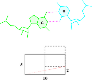
The blocview script in 3DNA has been created as a handy tool to effectively reveal key features of small to medium-sized nucleic acid structures. Specifically, the bloc part of the name means ‘block’, i.e., the rectangular block in Calladine-Drew style schematic representation to distinguish bases by size (larger purine vs. smaller pyrimidine), identity (red for A, yellow for C, green for G, and blue for T), and groove (minor edge in black). The view part stands for the most extended view, as defined by the principal axes of inertia. Implementation-wise, blocview calls several 3DNA utility programs and MolScript (for protein ribbons and nucleic acid backbone rods) to prepare the scenes, and then uses Raster3D (specifically, render) or PyMol to generate a PNG image.
The blocview script was originally written in Perl. As of 3DNA v2.1, I decided to switch the scripting language to Ruby for its consistent object-oriented style, succinct and flexible syntax. Previously available Perl scripts are now moved out of the default 3DNA executable directory $X3DNA/bin/ into $X3DNA/perl_scripts/. The blocview script has been re-written in Ruby and set as the default (at $X3DNA/bin/blocview); the original Perl version is renamed blocview.pl (at $X3DNA/perl_scripts/blocview.pl) to avoid confusion. The command line help message, available via blocview -h, is as below:
------------------------------------------------------------------------
Generate a schematic image which combines base block representation
with protein ribbon. The image has informative color coding for the
nucleic acid part and is set in the "best view" by default. Raster3D
(or PyMOL) and ImageMagick must be installed.
Usage:
blocview [options] PDBFile
Examples:
blocview -i 355d.png 355d.pdb
# generate image '355d.png'; display 355d.png
Options:
------------------------------------------------------------------------
--imgfile, -i <s>: name of image file (default: blocview.png)
--r3dfile, -r <s>: name of .r3d file (default: blocview.r3d)
--dpi-pymol, -d <i>: create PyMOL ray-traced image at specific DPI
--scale, -s <f>: set scale factor (for 'render' of Raster3D)
--xrot, -x <f>: rotation angle about x-axis
--yrot, -y <f>: rotation angle about y-axis
--zrot, -z <f>: rotation angle about z-axis
--original, -o: use original coordinates
--ball-and-stick, -b: get a ball-and-stick image
--p-base-ring, -c: use only P and base ring atoms
--no-ds, -n: do not show double-helix ribbon
--protein, -p: set best view based on protein atoms
--all, -a: set best view based on all atoms
--version, -v: Print version and exit
--help, -h: Show this message
Using the x-ray crystal structure of d(GGCCAATTGG) complexed with netropsin (1z8v) in the minor groove as an example, the command to run is as follows:
blocview -i 1z8v.png 1z8v.pdb
# The following two forms are also fine
# blocview --imgfile 1z8v.png 1z8v.pdb
# blocview --imgfile=1z8v.png 1z8v.pdb
# The Perl version can be run like this:
# $X3DNA/perl_scripts/blocview.pl -i=1z8v.png 1z8v.pdb
The image, named 1z8v.png, is shown below. Note that it is generated automatically from the PDB-formatted data file 1z8v.pdb. In this representation, one can see clearly that there are two unpaired Gs (green block) at each 5′-end of the two DNA chains (red and yellow rods), and a drug molecule (ball-and-stick) binds in the minor groove (black edge of the rectangular blocks). Moreover, the deformation in propeller and buckle is obvious in this schematic presentation.

Over the years, blocview-generated images have been used in NDB for virtually all nucleic acid structures (see for example, the NDB atlas gallery for x-ray drug-DNA complexes). It’s worth noting that such simple images have also be adopted by the RCSB PDB, prominently at the summary page, for nucleic acid containing structures (see PDB entry 1z8v). Given the effectiveness of blocview-generated schematic representation and its adoption by the NDB and PDB, I’m hopeful that blocview will be more widely used by the general DNA/RNA structure community. As always, I value user’s feedback in continuously refining the script.
One of 3DNA’s unique features is the simplified rectangular block representation of bases and base-pairs, as shown in the figure below. This type of schematic depiction was first made popular by Calladine and Drew (see their book titled Understanding DNA — The Molecule & How It Works), thus I usually call it the Calladine-Drew style representation.

By default, a base-pair [BP, (a)] has dimensions of 10×4.5×0.5 (Å); a purine [R, (b) left] 4.5×4.5×0.5 (Å); a pyrimidine [Y, (b) right] 3×4.5×0.5 (Å); and a mean base [M, (c)], which is exactly half of the base-pair, 5×4.5×0.5 (Å).
The blocks are stored into separate files: Block_BP.alc, Block_R.alc, and Block_Y.alc for BP, R and Y respectively. To use M for R and Y (i.e., set R and Y to be of equal size), simple copy file Block_M.alc to overwrite Block_R.alc and Block_Y.alc in the current working directory for local effect, or the 3DNA installation directory ($X3DNA/config/) for global impact. These blocks are used in the rebuilding and visualization components of 3DNA.
Following SCHNArP, 3DNA uses alchemy, a simple chemical file format, to specify explicitly the nodes (atoms) and edges (bonds) of a rectangular block. Three file formats (alchemy, MDL molfile, and Tripos mol2), supported by RasMol v2.6 (the most popular molecular graphics visualization program in the 1990s), serve the purpose of specifying the rectangular block. I cannot recall exactly why I picked up -alchemy instead of -mdl and -mol2, perhaps because of its simplicity: I played around with sample alchemy files and came up with the alchemy rectangular block files used by SCHNArP, without much difficulty.
As an example, Block_BP.alc has the following content:
12 ATOMS, 12 BONDS
1 N -2.2500 5.0000 0.2500
2 N -2.2500 -5.0000 0.2500
3 N -2.2500 -5.0000 -0.2500
4 N -2.2500 5.0000 -0.2500
5 C 2.2500 5.0000 0.2500
6 C 2.2500 -5.0000 0.2500
7 C 2.2500 -5.0000 -0.2500
8 C 2.2500 5.0000 -0.2500
9 C -2.2500 5.0000 0.2500
10 C -2.2500 -5.0000 0.2500
11 C -2.2500 -5.0000 -0.2500
12 C -2.2500 5.0000 -0.2500
1 1 2
2 2 3
3 3 4
4 4 1
5 5 6
6 6 7
7 7 8
8 5 8
9 9 5
10 10 6
11 11 7
12 12 8
Observant viewers may notice that nodes 1-4 are specified as nitrogens (N) which have exactly the same coordinates as 9-12 (carbons, C). This is a little trick to make RasMol display the minor groove edge in a different color (blue for N) than the other five sides of the rectangular (gray for C), as shown in the following figure:

Note that the rectangular is preset in the standard base reference frame. Thus the nodes have y-coordinates of +5 Å and -5 Å along the long edge of the base pair, and x-coordinates of +2.25 Å and -2.25 Å along the short edge.
As an extra bonus of storing the rectangular blocks in external alchemy text files, the dimensions of the blocks can be readily changed. For example, the thickness of a block (z-coordinates) can be easily increased from 0.5 to 1.0 Å to make it thicker. Moreover, the blocks do not need to be rectangular either — they can appear to be triangular blocks.
It’s worth noting that while extensively used in 3DNA for schematic representations, the alchemy format has largely become a legacy in cheminformatics/bioinformatics nowadays. Searching the internet, I cannot find the specification of the format. Moreover, the support of alchemy is quite limited and buggy in molecular graphics visualization programs most widely used today: PyMOL does not understand this format at all; RasMol v2.7 has a bug in interpreting it; only Jmol can properly read 3DNA base-pair rectangular block files in alchemy [see initial discussion and follow-up]. To resolve the issues associated with alchemy format, and thus to make 3DNA base-pair block schematics more widely available, I have recently added a converter in v2.1 to readily transform alchemy to MDL molfile, a format consistently supported by PyMOL, Jmol and RasMol. I’ll talk about this feature in another post.
The conformation of the five-membered sugar ring in DNA/RNA structures can be characterized by the five consecutive endocyclic torsion angles (see Figure below), i.e.,
ν0: C4′-O4′-C1′-C2′
ν1: O4′-C1′-C2′-C3′
ν2: C1′-C2′-C3′-C4′
ν3: C2′-C3′-C4′-O4′
ν4: C3′-C4′-O4′-C1′
Due to the ring constraint, the conformation can be characterized approximately by 5-3=2 parameters. Using the concept of pseudorotation of the sugar ring, the two parameters are the amplitude (τm) and phase angle (P).
One set of widely used formula to convert the five torsion angles to the pseudorotation parameters is due to Altona & Sundaralingam (1972): Conformational Analysis of the Sugar Ring in Nucleosides and Nucleotides. A New Description Using the Concept of Pseudorotation [J. Am. Chem. Soc., 94(23), pp. 8205–8212]. The concept is easily illustrated with an example — here with the G4 sugar ring on chain A of the Dickerson dodecamer (1bna), using Octave/Matlab code:
# xyz coordinates of the G4 sugar ring on chain A of 1bna
# ATOM 63 C4' DG A 4 21.393 16.960 18.505 1.00 53.00
# ATOM 64 O4' DG A 4 20.353 17.952 18.496 1.00 38.79
# ATOM 65 C3' DG A 4 21.264 16.229 17.176 1.00 56.72
# ATOM 67 C2' DG A 4 20.793 17.368 16.288 1.00 40.81
# ATOM 68 C1' DG A 4 19.716 17.901 17.218 1.00 30.52
# endocyclic torsion angles:
v0 = -26.7; v1 = 46.3; v2 = -47.1; v3 = 33.4; v4 = -4.4;
Pconst = sin(pi/5) + sin(pi/2.5); # 1.5388
P0 = atan2(v4 + v1 - v3 - v0, 2.0 * v2 * Pconst); # 2.9034
tm = v2 / cos(P0) # amplitude: 48.469
P = 180/pi * P0 # phase angle: 166.35 [P + 360 if P0 < 0]
The Altona & Sundaralingam (1972) pseudorotation parameters are what have been adopted in 3DNA. The Curves+ program, on the other hand, uses another set of formula due to Westhof & Sundaralingam (1983): A Method for the Analysis of Puckering Disorder in Five-Membered Rings: The Relative Mobilities of Furanose and Proline Rings and Their Effects on Polynucleotide and Polypeptide Backbone Flexibility. [J. Am. Chem. Soc., 105(4), pp. 970–976]. The two sets of formula — Altona & Sundaralingam (1972) and Westhof & Sundaralingam (1983) — give slightly different numerical values for the two pseudorotation parameters (see below).
Since Curves+ and 3DNA are currently the most commonly used programs for conformational analysis of nucleic acid structures, the subtle differences in these two pseudorotation parameters may cause confusions for users who use both programs. With the same G4 (on chain A of 1bna) sugar ring, here is the Octave/Matlab script showing how Curve+ calculates the pseudorotation parameters:
# xyz coordinates of the G4 sugar ring on chain A of 1bna
# endocyclic torsion angles, same as above
v0 = -26.7; v1 = 46.3; v2 = -47.1; v3 = 33.4; v4 = -4.4;
v = [v2, v3, v4, v0, v1]; # reorder them into vector v[]
A = 0; B = 0;
for i = 1:5
t = 0.8 * pi * (i - 1);
A += v(i) * cos(t);
B += v(i) * sin(t);
end
A *= 0.4; # -48.476
B *= -0.4; # 11.516
tm = sqrt(A * A + B * B); # 49.825
c = A/tm; s = B/tm;
P = atan2(s, c) * 180 / pi; # 166.64
For this specific example, i.e., the G4 sugar ring on chain A of 1bna, the pseudorotation parameters as calculated by 3DNA following Altona & Sundaralingam (1972) and Curves+ following Westhof & Sundaralingam (1983) are as follows:
|
amplitude (τm) |
phase angle (P) |
| 3DNA |
48.469 |
166.35 |
| Curves+ |
49.825 |
166.64 |
Needless to say, for the majority of cases like the one shown here, the differences are subtle; very few people would notice them or be bothered at all. For those who do care about such little details, however, this post shows where the discrepancies really come from.
In the field of nucleic acid structural analysis, it seems fair to say that Curves+ and 3DNA are nowadays the top two choices. To the best of my knowledge, these two programs are also the only ones that confirm to the standard base reference frame. Moreover, as noted in my previous post, Curves+ and 3DNA are “constructive competitors” with complementary functionality: Curves+ is unique in providing a curvilinear helical axis, a bending analysis, a full description of groove widths and depths and its seamless integration to the analysis of molecular dynamics trajectories, while 3DNA’s strength lies in its cohesrent approach combining analysis, rebuilding, and visualization into one package.
Given the complementarity between Curve+ and 3DNA, it makes sense to build a ‘bridge’ between the two so users can easily take advantage of both programs. Starting from 3DNA v1.5, find_pair has the -c option to generate input for Curves directly from a PDB file. Over the years, this option appears to have received little attention — at least, I am not aware of any literature reference to it. Now, the updated Curves+ program has introduced the new lib name list variable, among other changes. I have thus added the -curves+ option (abbreviation -c+) to find_pair to make its output compatible with Curves+.
As always, the point/process is best illustrated with an example — here with the Dickerson B-DNA dodecamer solved at high resolution by Williams et al. (PDB entry 355d).
find_pair -c+ 355d.pdb 355d-curves+.inp
The generated file 355d-curves+.inp has the following content:
&inp file=355d.pdb,
lis=355d,
fit=.t.,
lib=/Users/xiangjun/Curves+/standard,
isym=1,
&end
2 1 -1 0 0
1 2 3 4 5 6 7 8 9 10 11 12
24 23 22 21 20 19 18 17 16 15 14 13
which can be fed into Curves+ as below,
Cur+ < 355d-curves+.inp
The four output files are: 355d.cda, 355d.lis, 355d_X.pdb and 355d_b.pdb.
Please note the followings:
- The environment variable CURVES_PLUS_STDLIB should be set, pointing to the directory where Curves+ is installed (containing files
standard_b.lib and standard_s.lib). In the example above, CURVES_PLUS_STDLIB is set to /Users/xiangjun/Curves+.
- The
find_pair -c+ option (currently) is applicable only to double helical DNA/RNA structures, the most common application scenario.
- The
-c+ option ignores HETATM records, in accordance with Curves+ where proteins, water and HETATM are automatically removed at input. (see Curves+ user manual, section Input data)
- To run
Cur+ < 355d-curves+.inp again in the same folder, the four output files must first be deleted (e.g., rm -f 355d.cda 355d.lis 355d_[Xb].pdb). This is best taken care of via a script.
Obviously, the nucleic acid structure community benefits the most to have both Curves+ and 3DNA at its disposal and be able to easily switch between them — hopefully, the find_pair -c+ option would serve as such a ‘bridge’.
From the very beginning, 3DNA calculates a set of nucleic acid backbone parameters, including the six main chain torsion angles (α, β, γ, δ, ε, and ζ) around the covalent bonds, χ about the glycosidic bond, and the sugar pucker (see figure below). For double helical structures, the standard analyze output (.out file) has a section for “Main chain and chi torsion angles,” and another dedicated to “Sugar conformational parameters”. Based on my experience/understanding, these two parts are well recognized and utlizied by 3DNA users. What has receive little attention (in spite of the several posts I’ve written on the topic), though, is 3DNA’s applicability to single-stranded (ss) RNA structures for the backbone torsions, among other parameters. Using the fully refined crystal structure of the Haloarcula marismortui large ribosomal subunit (PDB entry 1jj2) as an example, the procedure is below:
find_pair -s 1jj2.pdb 1jj2.nts
analyze 1jj2.nts
# or the above two steps can be combined:
find_pair -s 1jj2.pdb stdout | analyze stdin
# see output file '1jj2.outs'
In retrospect, the fact that 3DNA has been little used for RNA backbone conformational analysis is of no surprise:
- While base-pair parameters have different (oftentimes confusing) definitions, these backbone parameters are pretty “standard” — thus, for example, any program for DNA/RNA structural analysis would give the same numerical values for α or χ torsion angles.
- The two-step process as illustrated above is a bit awkward, and the torsions are “buried” among many other parameters.
- 3DNA is more directly “linked” (conceivably) to DNA base pairs than to RNA backbone.
So while adapting the Zp parameter for ss DNA/RNA structures in 3DNA v2.1, I also take this opportunity to add the -torsion option to analyze with the following handy features:
- Streamline the calculation by starting directly from a PDB file and output only backbone parameters. So the above example can be shortened to
analyze -t=1jj2.tor 1jj2.pdb; the output file is named 1jj2.tor.
- Classify backbone into BI/BII conformation, and base χ into syn / anti.
- Add pseudo-torsions, and Zp and Dp as defined by Richardson et al.
- Handle pseudouridine sensibly, and work also for nucleic acid structure with only backbone atoms.
- Be easy to use, efficient and robust — it takes ~1 second to process the large ribosomal subunit 1jj2 (with 2876 nucleotides consisting of 23S rRNA and 5S rRNA) on my MacBook Air.
Overall, analyze -torsion is designed to be pragmatic and allows for automatic processing of all NDB entries or molecular dynamics trajectories. Given below is an excerpt of the three sections from an analyze -torsion run on 1jj2:
****************************************************************************
Main chain and chi torsion angles:
Note: alpha: O3'(i-1)-P-O5'-C5'
beta: P-O5'-C5'-C4'
gamma: O5'-C5'-C4'-C3'
delta: C5'-C4'-C3'-O3'
epsilon: C4'-C3'-O3'-P(i+1)
zeta: C3'-O3'-P(i+1)-O5'(i+1)
chi for pyrimidines(Y): O4'-C1'-N1-C2
chi for purines(R): O4'-C1'-N9-C4
If chi is in range [-90, +90], syn conformation
otherwise, it is in anti conformation
e-z: epsilon - zeta
BI: e-z = [-160, +20]
BII: e-z = [+20, +200]
base chi alpha beta gamma delta epsilon zeta e-z
1 0:..10_:[..U]U -62.5(syn) --- --- 56.2 74.0 142.2 -87.8 -130.1(BI)
2 0:..11_:[..A]A 171.5(anti) 173.2 -161.0 168.5 84.0 -112.1 -65.4 -46.7(BI)
3 0:..12_:[..U]U -167.7(anti) -70.7 168.4 53.0 78.5 -128.5 -46.4 -82.1(BI)
4 0:..13_:[..G]G -172.5(anti) -61.8 170.4 67.7 73.5 -166.7 -79.6 -87.1(BI)
5 0:..14_:[..C]C -166.0(anti) -73.0 -172.5 55.1 83.2 -143.3 -77.7 -65.6(BI)
6 0:..15_:[..C]C -155.5(anti) -60.9 174.1 47.3 80.3 -154.4 -71.2 -83.2(BI)
****************************************************************************
Pseudo (virtual) eta/theta torsion angles:
Note: eta: C4'(i-1)-P(i)-C4'(i)-P(i+1)
theta: P(i)-C4'(i)-P(i+1)-C4'(i+1)
eta': C1'(i-1)-P(i)-C1'(i)-P(i+1)
theta': P(i)-C1'(i)-P(i+1)-C1'(i+1)
eta": Borg(i-1)-P(i)-Borg(i)-P(i+1)
theta": P(i)-Borg(i)-P(i+1)-Borg(i+1)
base eta theta eta' theta' eta" theta"
1 0:..10_:[..U]U --- --- --- --- --- ---
2 0:..11_:[..A]A -174.6 -129.7 177.0 -127.7 -157.5 -75.5
3 0:..12_:[..U]U 149.1 -105.1 174.1 -101.2 -111.0 -69.4
4 0:..13_:[..G]G 169.0 -172.5 -156.6 -169.2 -93.3 -137.1
5 0:..14_:[..C]C 176.2 -143.4 179.6 -140.6 -144.6 -120.6
6 0:..15_:[..C]C 165.0 -147.7 177.4 -146.8 -149.2 -121.7
****************************************************************************
Sugar conformational parameters:
Note: v0: C4'-O4'-C1'-C2'
v1: O4'-C1'-C2'-C3'
v2: C1'-C2'-C3'-C4'
v3: C2'-C3'-C4'-O4'
v4: C3'-C4'-O4'-C1'
tm: the amplitude of pucker
P: the phase angle of pseudorotation
Zp: z-coordinate of the 3' phosphorus atom (P) expressed in the
standard base reference frame; it's POSITIVE when P is on
the +z-axis side (base in anti conformation); NEGATIVE if
P is on the -z-axis side (base in syn conformation)
Dp: perpendicular distance of the 3' P atom to the glycosydic bond
[as per the MolProbity paper of Richardson et al. (2010)]
base v0 v1 v2 v3 v4 tm P Puckering Zp Dp
1 0:..10_:[..U]U -11.3 -15.4 34.5 -41.8 33.5 41.6 33.8 C3'-endo -0.13 3.53
2 0:..11_:[..A]A 11.4 -30.2 36.9 -31.5 12.6 36.9 1.2 C3'-endo 4.74 4.78
3 0:..12_:[..U]U 3.6 -29.3 42.4 -41.3 23.8 43.6 13.9 C3'-endo 4.67 4.82
4 0:..13_:[..G]G -13.0 -17.8 39.8 -47.9 38.5 47.8 33.7 C3'-endo 4.45 4.46
5 0:..14_:[..C]C 6.0 -28.4 38.9 -36.5 19.2 39.5 10.1 C3'-endo 4.57 4.70
6 0:..15_:[..C]C 1.9 -26.4 39.6 -39.6 23.7 41.2 16.0 C3'-endo 4.32 4.61
Given the x-, y-, and z-coordinates of four points (a-b-c-d) in 3-dimensional (3D) space, how to calculate the torsion angle? Overall, this is a well-solved problem in structural biology and chemistry; one can find a description of torsion angle in many text books and on-line documents. The algorithm for its calculation is implementated in virtually every software package in computational structural biology and chemistry.
As basic as the concept is, however, it is important (based on my experience) to have a clear understanding of how torsion angle is defined in order to really get into the 3D world. Here is a worked example using Octave/Matlab of my simplified, geometry-based implementation of calculating torsion angle, including how to determine its sign. No theory or (complicated) mathematical formula, just a step-by-step illustration of how I solve this problem.
- Coordinates of four points are given in variable
abcd:
abcd = [ 21.350 31.325 22.681
22.409 31.286 21.483
22.840 29.751 21.498
23.543 29.175 22.594 ];
- Two auxiliary functions: norm_vec() to normalize a vector; get_orth_norm_vec() to get the orthogonal component (normalized) of a vector with reference to another vector, which should have already been normalized.
function ovec = norm_vec(vec)
ovec = vec / norm(vec);
endfunction
function ovec = get_orth_norm_vec(vec, vref)
temp = vec - vref * dot(vec, vref);
ovec = norm_vec(temp);
endfunction
- Get three vectors: b_c is the normalized vector b→c; b_a_orth is the orthogonal component (normalized) of vector b→a with reference to b→c; c_d_orth is similarly defined, as the orthogonal component (normalized) of vector c→d with reference to b→c.
b_c = norm_vec(abcd(3, :) - abcd(2, :))
% [0.2703158 -0.9627257 0.0094077]
b_a_orth = get_orth_norm_vec(abcd(1, :) - abcd(2, :), b_c)
% [-0.62126 -0.16696 0.76561]
c_d_orth = get_orth_norm_vec(abcd(4, :) - abcd(3, :), b_c)
% [0.41330 0.12486 0.90199]
- Now the torsion angle is defined as the angle between the two vectors, b_a_orth and c_d_orth, and can be easily calculated by their dot product. The sign of the torsion angle is determined by the relative orientation of the cross product of the same two vectors with reference to the middle vector b→c. Here they are in opposite direction, thus the torsion angle is negative.
angle_deg = acos(dot(b_a_orth, c_d_orth)) * 180 / pi % 65.609
sign = dot(cross(b_a_orth, c_d_orth), b_c) % -0.91075
if (sign < 0)
ang_deg = -angle_deg % -65.609
endif
A related concept is the so-called dihedral angle, or more generally the angle between two planes. As long as the normal vectors to the two corresponding planes are defined, the angle between them is easy to work out.
It’s worth noting that the helical twist angle in SCHNAaP and 3DNA is calculated similarly.
Backbone conformation of nucleic acid structures is most characterized by a set of 6 torsion angles (α, β, γ, δ, ε, and ζ) around the consecutive chemical bonds, chi (χ) quantifying the relative base/sugar orientation, plus the sugar pucker.

This large number of DNA/RNA backbone conformational parameters is in striking contrast to the two torsion angles (φ and ψ) in protein structures, routinely employed in Ramachandran plot. Over the years, the nucleic acid community has come up with simplified ways to represent DNA/RNA backbone conformation. Thus far, the most widely used one is the pseudo-torsion angles (See figure below) η: C4′(i-1)-P(i)-C4′(i)-P(i+1) and θ: P(i)-C4′(i)-P(i+1)-C4′(i+1).

The history of the P—C4′ virtual-bond concept and its application in RNA structure analysis have recently been reviewed by Pyle et al. in A new way to see RNA [Q Rev Biophys. 2011, 44(4), 433—466], where the following three contributions are highlighted:
- Olson (1980). Configurational statistics of polynucleotide chains. An updated virtual bond model to treat effects of base stacking., Macromolecules 13(3), 721—728.
- Malathi & Yathindra (1980). A novel virtual bond scheme to probe ordered and random coil conformations of nucleic acids: Configurational statistics of polynucleotide chains. Current Science, 49, 803—807.
- Duarte & Pyle (1998). Stepping through an RNA structure: A novel approach to conformational analysis. Journal of Molecular Biology, 284, 1465—1478.
More recently, Pyle et al. also employed a modified version of the pseudo-torsions, η′: C1′(i-1)-P(i)-C1′(i)-P(i+1) and θ′: P(i)-C1′(i)-P(i+1)-C1′(i+1), i.e., using C1′ instead of C4′, and found that:
The η′ and θ′ torsions are more suitable when interpreting crystallographic density because the C1′ atom is covalently bound to the nucleoside base and therefore can be more easily and accurately located within a low-resolution map.
While implementing the -torsion option to analyze to make it more explicit that 3DNA readily calculates conventional backbone torsion angles, I also take this opportunity to add the pseudo-torsion angles — η/θ and η′/θ′, among other new parameters. Moreover, while I am at it, I cannot help but also compute yet another set of pseudo-torsion angles: η″/θ″. Here, instead of C1′ or C4′, the origin of the base reference frame is employed; it can be taken as a _pseudo_-atom more accurately defined by the base plane than any real single atom.
The usefulness of η″/θ″, especially in comparison with η/θ and η′/θ′, remains to be determined. However, only η″/θ″ uniquely takes advantage of the two most accurately determined entities in a nucleic acid structure, the heavy phosphorus atom and the rigid base plane [see discussion (p.16) in the Richardson et al. MolProbity paper, Acta Cryst. (2010). D66, 12–21] Presumably, η″/θ″ provides a new perspective in RNA structural analysis by combining the backbone and the base.
Here is the pseudo-torsions for the yeast phenylalanine transfer RNA (6tna by simply running analyze -torsion=6tna.tor 6tna.pdb):
Pseudo (virtual) eta/theta torsion angles:
Note: eta: C4'(i-1)-P(i)-C4'(i)-P(i+1)
theta: P(i)-C4'(i)-P(i+1)-C4'(i+1)
eta': C1'(i-1)-P(i)-C1'(i)-P(i+1)
theta': P(i)-C1'(i)-P(i+1)-C1'(i+1)
eta": Borg(i-1)-P(i)-Borg(i)-P(i+1)
theta": P(i)-Borg(i)-P(i+1)-Borg(i+1)
base eta theta eta' theta' eta" theta"
1 A:...1_:[..G]G --- -126.6 --- -141.5 --- -130.4
2 A:...2_:[..C]C 167.8 -168.3 174.6 -152.5 -151.4 -115.4
3 A:...3_:[..G]G 160.4 -119.8 -171.9 -138.9 -123.6 -119.2
4 A:...4_:[..G]G 148.0 -164.2 162.1 -159.2 -154.4 -124.6
5 A:...5_:[..A]A 168.7 -137.6 -175.9 -137.8 -129.5 -115.0
6 A:...6_:[..U]U 171.8 -145.7 -172.5 -140.5 -131.3 -124.7
7 A:...7_:[..U]U -151.0 -47.8 -136.0 -58.6 -117.7 -30.2
8 A:...8_:[..U]U 160.9 159.7 -161.0 -163.6 -144.2 178.0
9 A:...9_:[..A]A -137.0 -48.6 -158.1 -108.9 161.5 -104.7
10 A:..10_:[2MG]g 33.1 -135.8 93.4 -134.6 134.1 -113.0
11 A:..11_:[..C]C 167.2 -138.3 -179.4 -137.7 -142.4 -118.7
12 A:..12_:[..U]U 165.5 -120.7 -179.3 -128.0 -145.8 -106.7
13 A:..13_:[..C]C 174.1 -173.6 -165.5 179.6 -120.9 -180.0
14 A:..14_:[..A]A 173.0 -144.0 172.7 -132.4 177.6 -72.7
15 A:..15_:[..G]G 154.7 110.6 -176.2 85.5 -97.7 -76.9
16 A:..16_:[H2U]u 76.3 94.1 65.3 119.7 -152.8 -123.8
17 A:..17_:[H2U]u -36.7 -79.6 -50.7 -136.6 -142.7 -159.0
18 A:..18_:[..G]G -9.7 -166.8 41.7 -158.6 28.9 -120.4
19 A:..19_:[..G]G -131.6 -35.8 -122.9 -67.8 -104.3 -10.5
20 A:..20_:[..G]G 160.9 -93.2 -161.6 -98.9 -174.1 -112.3
21 A:..21_:[..A]A -83.6 152.5 -72.8 155.7 -59.1 155.4
22 A:..22_:[..G]G 164.1 169.4 160.0 -178.5 159.1 -157.6
23 A:..23_:[..A]A 177.6 -148.5 -174.5 -142.7 -154.5 -114.3
24 A:..24_:[..G]G 167.2 -98.9 -171.7 -128.6 -127.6 -99.1
25 A:..25_:[..C]C 151.6 -153.5 167.3 -140.8 -137.7 -84.8
26 A:..26_:[M2G]g 156.2 -137.4 -175.2 -135.2 -100.0 -104.2
27 A:..27_:[..C]C 166.2 -145.5 -177.9 -140.4 -129.1 -116.8
28 A:..28_:[..C]C 164.7 -140.5 175.8 -145.3 -152.7 -123.4
29 A:..29_:[..A]A 161.2 -145.3 175.7 -144.9 -142.0 -126.0
30 A:..30_:[..G]G -173.5 -120.3 -158.4 -133.2 -126.6 -94.4
31 A:..31_:[..A]A 169.8 -153.1 177.7 -140.4 -124.5 -81.5
32 A:..32_:[OMC]c 154.4 -126.8 -178.7 -131.3 -104.1 -128.0
33 A:..33_:[..U]U 170.0 -103.9 -179.9 -152.7 -164.6 143.6
34 A:..34_:[OMG]g -4.7 -123.7 41.8 -124.8 31.6 -99.6
35 A:..35_:[..A]A 163.5 -104.3 176.9 -127.9 -137.5 -128.2
36 A:..36_:[..A]A 175.9 173.6 180.0 -167.7 -156.4 -118.3
37 A:..37_:[.YG]g 166.8 -131.7 -174.5 -133.0 -115.1 -82.9
38 A:..38_:[..A]A 167.7 -121.6 -175.7 -114.3 -109.9 -79.9
39 A:..39_:[PSU]P 168.3 -146.8 -160.2 -146.4 -98.6 -116.5
40 A:..40_:[5MC]c 160.6 -138.7 174.0 -141.8 -139.7 -126.5
41 A:..41_:[..U]U 164.8 -161.4 175.9 -152.3 -150.5 -117.6
42 A:..42_:[..G]G 174.3 -140.9 -170.3 -145.4 -129.1 -121.3
43 A:..43_:[..G]G 169.6 -159.0 -176.2 -154.9 -133.7 -133.1
44 A:..44_:[..A]A 174.0 -121.5 -174.2 -122.0 -143.1 -74.9
45 A:..45_:[..G]G 174.4 -132.5 -166.2 -128.1 -101.8 -128.9
46 A:..46_:[7MG]g -112.8 -113.4 -127.2 -138.3 -139.8 -152.1
47 A:..47_:[..U]U -63.2 -53.8 -1.1 -92.0 22.8 -124.7
48 A:..48_:[..C]C -84.7 59.6 -20.1 8.9 19.3 -104.5
49 A:..49_:[5MC]c -56.8 -140.1 -29.9 -143.6 98.1 -125.4
50 A:..50_:[..U]U 173.6 -146.4 -178.3 -140.6 -147.6 -117.8
51 A:..51_:[..G]G 160.8 -148.1 -178.6 -150.7 -140.7 -121.9
52 A:..52_:[..U]U 164.9 -144.0 175.8 -143.5 -139.9 -114.3
53 A:..53_:[..G]G 168.2 -140.9 -171.1 -144.0 -121.6 -117.3
54 A:..54_:[5MU]u 167.0 -131.1 178.3 -124.9 -139.9 -77.0
55 A:..55_:[PSU]P 167.6 -114.2 -172.8 -155.6 -113.0 146.0
56 A:..56_:[..C]C 35.0 -121.5 52.6 -126.2 26.5 -83.8
57 A:..57_:[..G]G 168.4 -148.1 -177.1 -131.1 -115.4 -111.7
58 A:..58_:[1MA]a -136.3 -133.3 -106.5 -176.7 -105.3 149.6
59 A:..59_:[..U]U 23.0 -130.9 33.0 -115.4 48.2 -68.2
60 A:..60_:[..C]C -163.6 -54.3 -123.2 -76.4 -79.6 -36.4
61 A:..61_:[..C]C 125.5 -153.3 169.7 -144.7 -153.8 -123.4
62 A:..62_:[..A]A 172.5 -139.3 -177.0 -137.6 -150.7 -114.6
63 A:..63_:[..C]C 165.8 -146.6 -178.5 -149.8 -139.2 -127.8
64 A:..64_:[..A]A 164.7 -144.9 176.5 -145.8 -145.3 -118.1
65 A:..65_:[..G]G 170.4 -152.3 -175.5 -151.5 -132.3 -122.1
66 A:..66_:[..A]A 168.0 -152.0 -177.4 -150.2 -133.0 -118.7
67 A:..67_:[..A]A 170.9 -141.8 -178.4 -140.4 -134.8 -123.1
68 A:..68_:[..U]U 164.8 -135.1 -178.9 -137.9 -143.7 -95.2
69 A:..69_:[..U]U 168.2 -154.9 -174.3 -157.1 -112.2 -144.8
70 A:..70_:[..C]C 160.6 -153.2 170.7 -153.5 -164.4 -125.1
71 A:..71_:[..G]G 161.8 -144.3 172.1 -143.1 -145.7 -124.2
72 A:..72_:[..C]C 176.7 -136.4 -169.3 -134.5 -134.9 -87.1
73 A:..73_:[..A]A 160.6 -142.8 -179.7 -139.7 -112.8 -104.4
74 A:..74_:[..C]C -176.9 -115.9 -163.1 -115.4 -117.2 -68.7
75 A:..75_:[..C]C 169.8 80.9 -170.0 74.9 -108.5 -91.3
76 A:..76_:[..A]A --- --- --- --- --- ---
In nucleic acid structures, the chi (χ) torsion angle is about the glycosidic bond (N-C1′) that connects the sugar and the A/C/G/T/U bases (or their modified variants). Specifically, for pyrimidines (C, T and U), χ is defined by O4′-C1′-N1-C2; and for purines (A and G) by O4′-C1′-N9-C4 (see figure below).

Pseudouridine (5-ribosyluracil, PSU) was the first identified modified nucleoside in RNA and is the most abundant. PSU is unique in that it has a C-glycosidic bond (C-C1′) instead of the N-glycosidic bond common to all other nucleosides, canonical or modified. It thus poses a problem as to how to calculate the χ torsion angle: should it be O4′-C1′-C5-C4, reflecting the actual glycosidic bond connection, or should the conventional definition O4′-C1′-N1-C2 still be applied literally? As a concrete example, the figure below shows the (slightly) different numerical values (–162.7° vs. –163.9°), as given by the two definitions, for PSU 6 on chain A of the PDB entry 3cgp (based on the 2009 Biochemistry article by Lin & Kielkopf titled X-ray structures of U2 snRNA-branchpoint duplexes containing conserved pseudouridines).
Needless to say, the specific definition of the χ torsion angle for PSU in RNA structures is a very subtle point, and I am not aware of any discussion on this issue in literature. In 3DNA, PSU is identified explicitly, and χ is defined by O4′-C1′-C5-C4. In NDB and a couple of other tools I am familiar with, χ for PSU is defined by O4′-C1′-N1-C2. Again using 3cgp (figure below) as an example, 3DNA gives –162.7°, whilst NDB gives –163.9°. Additionally, this distinction in N-C1′ vs. C-C1′ connection also comes into play when calculating the perpendicular distance from the 3′ phosphorus atom to the glycosidic bond, as per Richardson et al.
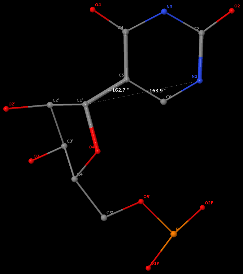
Except for pseudouridine, a nucleoside in DNA/RNA contains an N-glycosidic bond that connects the base to the sugar. The chi (χ) torsion angle, which characterizes the relative base/sugar orientation, is defined by O4′-C1′-N1-C2 for pyrimidines (C, T and U), and O4′-C1′-N9-C4 for purines (A and G).
Normally (as in A- and B-form DNA/RNA duplex), χ falls into the ranges of +90° to +180°; –90° to –180° (or 180° to 270°), corresponding to the anti conformation (Figure below, top). Occasionally, χ has values in the range of –90° to +90°, referring to the syn conformation (Figure below, bottom). Note that in left-handed Z-DNA with CG repeating sequence, the purine G is in syn conformation whilst the pyrimidine C is anti.
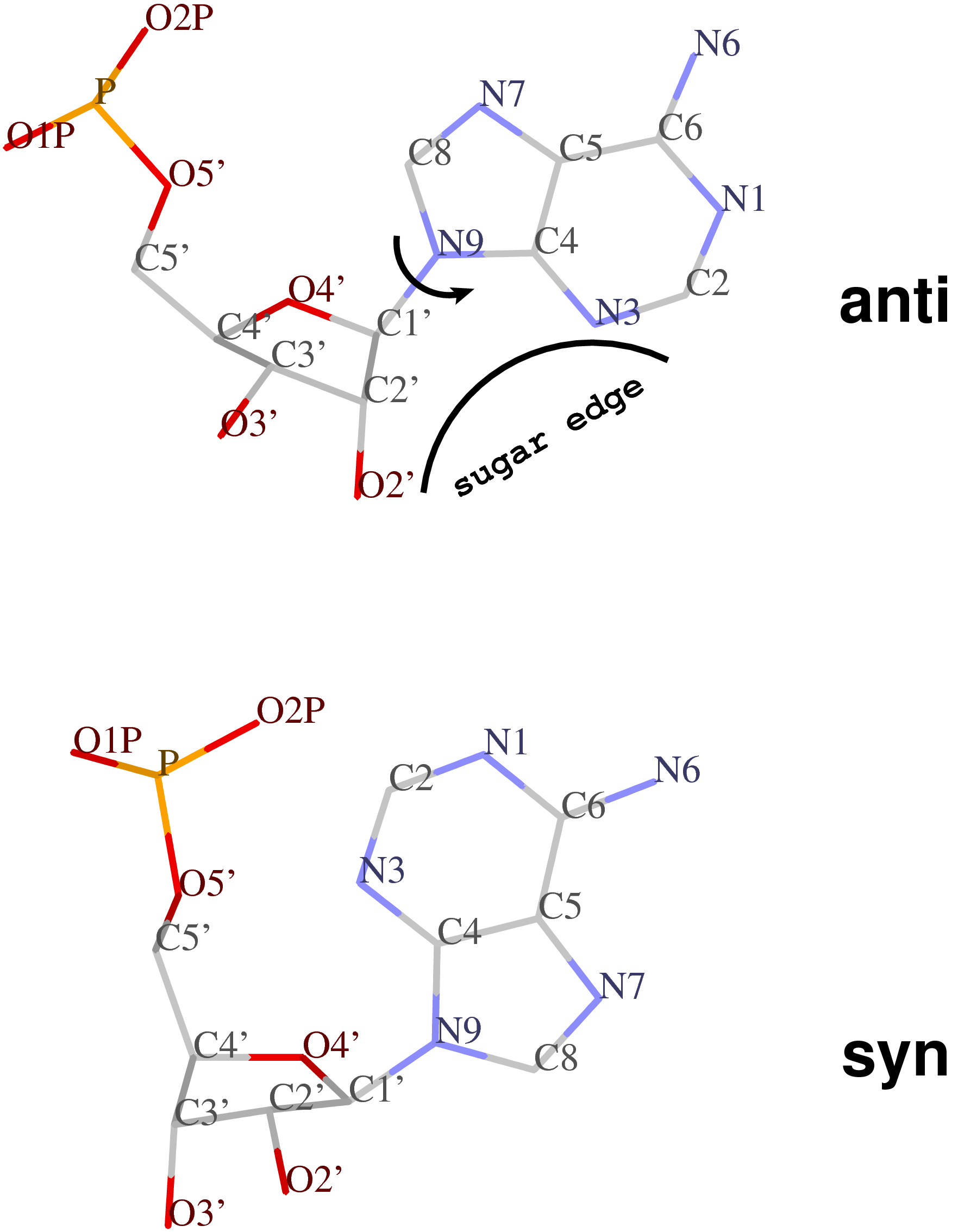
Presumably, the χ-related anti / syn conformation is a simple geometric concept. Nevertheless, the N-glycosidic bond and the corresponding χ torsion angle illustrate that the base and the sugar are two separate entities, i.e. there is an internal degree of freedom between them. In this respect, it is worth noting that the Leontis-Westhod sugar edge for base-pair classification corresponds to the anti form (as applied to RNA) only. When a base is flipped over into the syn conformation, the “sugar edge”, defined in connection with the minor (shallow) groove side of a nitrogenous bases, simply does not exist.
Base-flipping (anti / syn conformation switch) is one of the factors associated with the two possible relative orientations of the two bases in a pair, characterized explicitly in 3DNA as of type M+N or M–N since the 2003 NAR paper (Figure 2, linked below). I re-emphasized this distinction in our 2010 GpU dinucleotide platform paper (in particular, see supplementary Figure S2). Unfortunately, this subtle (but crucial, in my opinion) point has never been taken seriously (or at all) by the RNA community, even with 3DNA’s wide adoption. However, as people know 3DNA deeper/better and take RNA base-pair classification more rigorously, I have no doubt that the simplicity of this explicit distinction and the resultant full quantification of each and every possible base pair using standard geometric parameters will gradually be appreciated.
As of 3DNA v2.1, the output of the χ torsion angle is also associated with its classification in anti / syn conformation, among other new features (see for example the output for 6tna).
The sugar puckers in DNA/RNA structures are predominately in either C3′-endo (A-DNA or RNA) or C2′-endo (B-DNA; see Figure below, left), corresponding to the A- or B-form conformation in a duplex. In these two sugar conformations, the distance between neighboring phosphorus (P) atoms and the orientation of P relative to the sugar/bases are also dramatically different (figure below, right).
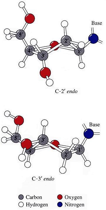
Recently, I carefully re-read some articles on RNA backbone conformation by Richardson et al., including:
I became intrigued by one of their observations: i.e., the correlation between the sugar pucker and a simple distance parameter:
C3′-endo and C2′-endo sugar puckers are highly correlated to the perpendicular distance between the C1′–N1/9 glycosidic bond vector and the following phosphate: > 2.9 Å for C3′-endo and < 2.9 Å for C2′-endo. (p.16 from the MolProbity paper).
Out of curiosity and for a better understanding of this correlation, I played around with some sample cases both visually and numerically. Overall, this involves a simple geometric calculation, i.e., the shortest distance from a point to a line in three-dimensional space. Given below is the Octave/Matlab script for calculating the distances for G175 and U176 of PDB entry 1jj2 (the large ribosomal subunit of Haloarcula marismortui):
function d = get_p3_nc_dist(P3, C1, N)
C1_N = N - C1; # vector from C1′ to N
nv_C1_N = C1_N / norm(C1_N); # normalized vector
C1_P3 = P3 - C1; # vector from C1′ to P3
proj = dot(C1_P3, nv_C1_N);
d = norm(C1_P3 - proj * nv_C1_N);
end
## G175
P3 = [70.104 112.366 44.586];
C1 = [73.017 109.666 45.304];
N9 = [74.445 109.380 45.288];
d1 = get_p3_nc_dist(P3, C1, N9) # 2.2 Å -- C2′-endo
## U176
P3 = [66.871 116.402 46.804];
C1 = [68.213 112.454 49.279];
N1 = [69.678 112.480 49.438];
d2 = get_p3_nc_dist(P3, C1, N1) # 4.6 Å -- C3′-endo
The GpU dinucleotide used in the above example forms a platform (see figure below), where the sugar of G175 adopts a C2′-endo conformation, and that of U176 C3′-endo. Indeed, the distance for G175 is 2.2 Å (< 2.9 Å); whilst the value for U176 is 4.6 Å (> 2.9 Å).
Note that the Richardson et al. articles focus on the RNA backbone, without paying attention to the base (pair) geometry. The 3DNA Zp parameter, which is the mean z-coordinate of the two P atoms in the mean reference frame of a dinucleotide step (see figure below), has been readily adapted to single-stranded RNA structures. For example, the vertical distances of the 3′ P atoms to the G175 and U176 base planes are 1.9 Å and 4.4 Å, respectively. Since base planes and the P atoms are the two most accurately located entities in a given nucleic acid structure, the nucleotide-based Zp variant is presumably more robust and discriminative than the distance from P to the glycosidic bond.
This new single-stranded based “Zp” parameter is available as of 3DNA v2.1.
RNA has three salient structural features (compared to DNA): it contains the ribose (not deoxyribose) sugar, it has the uracil (not thymine) base, and it is normally single (not double)-stranded. The O2′(G)…O2P(U) H-bond stabilized GpU dinucleotide platform may turn out to be the smallest unit with all those RNA hallmarks.
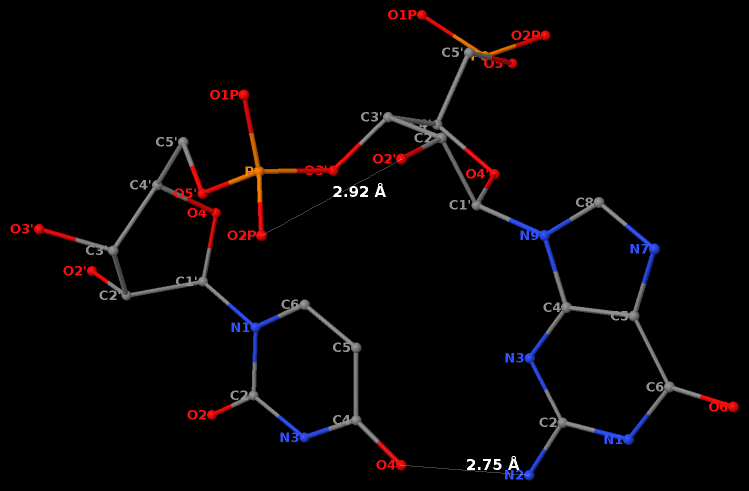
First, it must have the guanosine ribose to have the 2′-hydroxyl group form the O2′(G)…O2P(U) H-bond.
Second, the methyl group in position 5 of thymine would cause steric clash with guanosine, thus disrupting the N2(G)…O4(U) base-base H-bond to form the GpU dinucleotide platform.
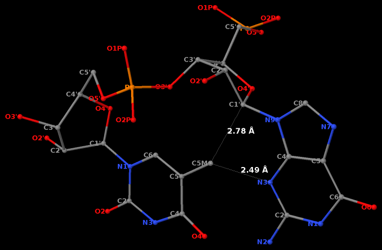
Third, a dinucleotide, by definition, is single-standed. The two H-bonds, plus the covalent linkage, makes the GpU platform extremely rigid (see Figure 1 of our 2010 NAR paper).
Moreover, the GpU platform is directional: swapping the two bases while keeping the sugar-phosphate backbone fixed does not allow for a base-base H-bond, thus no UpG dinucleotide platform.
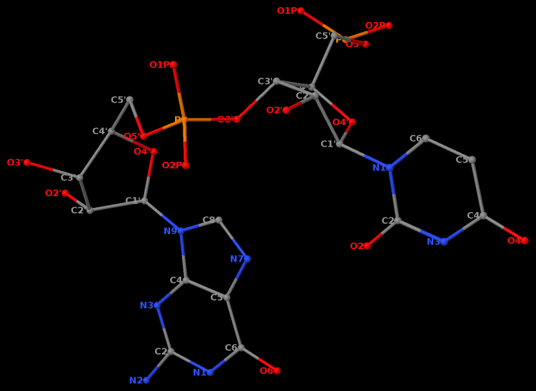
It worth noting that state-of-the-art quantum chemistry calculations have verified the importance of the O2′(G)…O2P(U) H-bond in stabilizing the GpU dinucleotide platform.
The least-squares (LS) fitting procedures presented below make use of well known mathematics. Indeed, the methods are so well known and widely used that it is somewhat difficult to locate the original references. In our previous effort to resolve the discrepancies among nucleic acid conformational analysis programs, we came across a variety of LS fitting procedures. Here we provide a detailed description, with step-by-step examples, of our implementation in 3DNA of two LS fitting algorithms based on a covariance matrix and its eigen-system. This post is the revised version of a note first made available in the “Technical Details” section of earlier 3DNA websites.
LS fitting between standard and experimental bases
Three analysis schemes — CompDNA, Curves/Curves+, and RNA — use LS procedures to fit a standard base with an embedded reference frame to an observed base structure. CompDNA and Curves/Curves+ take advantage of the conventional approach of McLachlan [“Least Squares Fitting of Two Structures.” J. Mol. Biol., 128, 74-79 (1979)], while the RNA program implements a closed-form solution of absolute orientation using unit quaternions first introduced by Horn. The two algorithms are mathematically equivalent for the most general cases, since the unit quaternion can be transformed to the rotation matrix given by McLachlan. The Horn method, however, is more straightforward and generally applicable; it can be applied even when one or both of the structures are perfectly planar, whereas the McLachlan approach fails.
Here we use the ideal adenine geometry derived from the high resolution crystal structures of model nucleosides, nucleotides, and bases. The x-, y-, and z-coordinates of the standard base, taken from the NDB, are listed below in the columns labeled sx, sy, and sz, respectively. s_(average) is the geometric center of the base.
sx sy sz
1 N9 0.213 0.660 1.287
2 C4 0.250 2.016 1.509
3 N3 0.016 2.995 0.619
4 C2 0.142 4.189 1.194
5 N1 0.451 4.493 2.459
6 C6 0.681 3.485 3.329
7 N6 0.990 3.787 4.592
8 C5 0.579 2.170 2.844
9 N7 0.747 0.934 3.454
10 C8 0.520 0.074 2.491
------------------------------------
s_(average): 0.4589 2.4803 2.3778
We similarly describe the coordinates of one of the adenine bases (the fifth nucleotide in the sequence strand) from the high resolution (1.4 Å) self-complementary d(CGCGAATTCGCG) dodecamer duplex determined by Williams and co-workers (PDB id: 355d). The experimental xyz coordinates are listed below in the columns labeled ex, ey, and ez. The geometric center is e_(average). Note that the atomic serial numbers from the PDB (first column) have been rearranged so that the atoms are in the same order as those of the ideal base listed above.
ex ey ez
91 N9 16.461 17.015 14.676
100 C4 15.775 18.188 14.459
99 N3 14.489 18.449 14.756
98 C2 14.171 19.699 14.406
97 N1 14.933 20.644 13.839
95 C6 16.223 20.352 13.555
96 N6 16.984 21.297 12.994
94 C5 16.683 19.056 13.875
93 N7 17.918 18.439 13.718
92 C8 17.734 17.239 14.207
------------------------------------
e_(average):16.1371 19.0378 14.0485
We collect the two sets of xyz coordinates in the 10 × 3 matrices S and E corresponding respectively to the standard and experimental bases. We then construct the 3 × 3 covariance matrix C between S and E using the following formula:
1 1
C = ------- [S' E - --- S' i i' E]
n - 1 n
=
0.2782 0.2139 -0.1601
-1.4028 1.9619 -0.2744
1.0443 0.9712 -0.6610
Here n, the number of atoms in each base, is 10, and i is an n x 1 column vector consisting of only ones. S' and i' are the transpose of matrix S and column vector i, respectively.
From the nine elements of the C matrix, we subsequently generate the 4 × 4 real symmetric matrix M using the expression:
| c11+c22+c33 c23-c32 c31-c13 c12-c21 |
M = | c23-c32 c11-c22-c33 c12+c21 c31+c13 |
| c31-c13 c12+c21 -c11+c22-c33 c23+c32 |
| c12-c21 c31+c13 c23+c32 -c11-c22+c33 |
=
1.5792 -1.2456 1.2044 1.6167
-1.2456 -1.0228 -1.1890 0.8842
1.2044 -1.1890 2.3447 0.6968
1.6167 0.8842 0.6968 -2.9011
The largest eigenvalue of matrix M is 4.0335, and its corresponding unit eigenvector is:
[ q0 q1 q2 q3 ] = [ 0.6135 -0.2878 0.7135 0.1780 ]
The rotation matrix R is deduced from the above eigenvector as below:
| q0q0+q1q1-q2q2-q3q3 2(q1q2-q0q3) 2(q1q3+q0q2) |
R = | 2(q2q1+q0q3) q0q0-q1q1+q2q2-q3q3 2(q2q3-q0q1) |
| 2(q3q1-q0q2) 2(q3q2+q0q1) q0q0-q1q1-q2q2+q3q3 |
=
-0.0817 -0.6291 0.7730
-0.1923 0.7710 0.6072
-0.9779 -0.0990 -0.1839
Following coordinate transformation with matrix R, the origin of the standard base is found to be displaced from the experimental structure by:
o = e_(average) - s_(average) R' = [15.8969 15.7701 15.1802]
The least-squares fitted coordinates (F) of the standard base atoms on the experimental structure are then given by:
F = S R' + i o
=
16.4592 17.0194 14.6699
15.7747 18.1925 14.4586
14.4899 18.4519 14.7542
14.1729 19.6974 14.4070
14.9343 20.6404 13.8420
16.2222 20.3472 13.5569
16.9832 21.2875 12.9925
16.6829 19.0585 13.8760
17.9183 18.4437 13.7219
17.7335 17.2396 14.2062
Here S is the (n x 3) matrix of original coordinates of the standard base, and as noted above, i is an n x 1 column vector consisting of only ones.
The difference matrix (D) between F and E, the (n x 3) matrix of original coordinates of the experimental base, and the root-mean-square (RMS) deviation between the two structures are found as:
D = E - F
=
0.0018 -0.0044 0.0061
0.0003 -0.0045 0.0004
-0.0009 -0.0029 0.0018
-0.0019 0.0016 -0.0010
-0.0013 0.0036 -0.0030
0.0008 0.0048 -0.0019
0.0008 0.0095 0.0015
0.0001 -0.0025 -0.0010
-0.0003 -0.0047 -0.0039
0.0005 -0.0006 0.0008
RMS deviation = 0.0054
It should be noted that if the standard base is already defined in terms of its reference frame, as in 3DNA (e.g., $X3DNA/config/Atomic_A.pdb), the vector o and the matrix R represent the best-fitted coordinate frame of the experimental base. Moreover, the three axes of the frame given by R are guaranteed to be orthonormal. If you want to get an insight of the LS fitting algorithm and a better understanding of how 3DNA derives its base reference frame, it’d be a valuable experience to repeat the above procedure with $X3DNA/config/Atomic_A.pdb.
Note: the algorithm does not apply to a molecule vs its inversion (an improper rotation) — thanks to Boris Averkiev for reporting this subtle point (see comments below). One possible remedy is to treat this edge case separately.
Base normal
Rather than fit a standard base to experimental coordinates, the CEHS, FREEHELIX, and NUPARM analyses perform a fitting of a LS plane to a set of atoms in order to define the base and base-pair normals. The covariance matrix based on the n x 3 matrix of experimental Cartesian coordinates E is diagonalized to find the vector normal to the best plane. Specifically, C is obtained using the above formula with S substituted by E. The normal vector then lies along the eigenvector that corresponds to the smallest eigenvalue. Note that the coefficient 1/(n-1) in the formula for calculating C has no effect on the direction of the eigenvectors but scales the magnitudes of the eigenvalues.
Using the above adenine base from the high resolution dodecamer duplex as an example, the covariance matrix C is:
C =
1.6680 -0.5015 -0.3253
-0.5015 2.0670 -0.5840
-0.3253 -0.5840 0.3061
The smallest eigenvalue of C, 8.26e-5, indicates that the base is almost perfectly planar. The corresponding unit eigenvector corresponding to the base normal is:
Base normal: 0.2737 0.3224 0.9062
Related topics:
As the old saying goes, a picture is worth a thousand words. To help you have a better idea of what 3DNA/DSSR is about, we’ve collected the following pictures; they serve to demonstrate selected features from 3DNA/DSSR’s versatile functionality.
Schematic diagram of base-pair parameters
Influence of Slide and Roll on DNA helical conformation

Roll-introduced DNA bending

Global bending of DNA associated with selective B → A conformational transformation

Canonical fiber models of A-, B-, C- and Z-DNA

3DNA-generated view of a four-way DNA–RNA junction (1egk)
.")
3DNA-detected pentaplets in the large ribosomal subunit (1jj2)
.")
−O2P(U) H-bond")
Nucleic-acid-containing structures generated with w3DNA

Analysis of DNA with a B-Z junction (2acj, left) and detection of hydration patterns (right)

Schematics images auto-generated via blocview
Over the years, the fiber utility program has become a handy way to generate standard B-DNA and A-DNA structures, as evident from citations to 3DNA. Nevertheless, the currently collected 55 experimental fiber models, comprehensive as they are, do not include one for canonical double-stranded (ds) RNA or single-stranded (ss) RNA structures of generic A/C/G/U sequence.
This situation is best illustrated by a recent article by Charles Brooks and Hashim Al-Hashimi and their co-workers, titled Unraveling the structural complexity in a single-stranded RNA tail: implications for efficient ligand binding in the prequeuosine riboswitch [Nucleic Acids Research, 40(3) 1345–1355 (2012)] , where they wrote:
Idealized A-form structures were constructed using Insight II (Molecular Simulations, Inc.) correcting the propeller twist angles from +15° to –15° using an in-house program, as previously described (47). The complementary strand was removed and the resulting ssRNA used in NMR data analysis. B-form helices were constructed using W3DNA (48).
As of 3DNA v2.1, however, that’s no longer the case: now the fiber utility provides direct support for generating idealized dsRNA or ssRNA structures of arbitrary A/C/G/U sequence. As always, the new functionality can be best illustrated with examples. Let’s build ssRNAs of the wild-type (5’-AUAAAAAACUAA-3’) and A29C mutated form (5’-AUAACAAACUAA-3’) used in the work cited above:
fiber -r -s -seq=AUAAAAAACUAA wt-12nt.pdb
fiber -r -s -seq=AUAACAAACUAA mt-12nt.pdb
Here the -r option is for RNA, -s for a ss structure, and -seq for the specific base sequence. The generated ssRNA structure for the wild-type sequence is named wt-12nt.pdb, and that for the mutated sequence named mt-12nt.pdb.
Note that the new RNA model is based on Struther Arnott’s work of fiber A-DNA from calf thymus (#1 in the list). The dsRNA, as its dsDNA counterpart, has a helical twist of 32.7° and a helical rise of 2.548 Å. Relevant to the above citation, here the propeller twist angle of each base pair is –10.5°, a negative value similar to that observed in high-resolution x-ray crystal structures. Furthermore, you can easily verify the three numbers with the following commands:
fiber -r -seq=AUAAAAAACUAA wt-12nt.pdb
find_pair wt-12nt.pdb stdout | analyze stdin
In summary, it is very easy to generate canonical RNA structures with the revised fiber command. Through its integrated analysis routine, 3DNA can also be used to check structural features of the resultant RNA models. Moreover, as mentioned in the opening post What can 3DNA do for RNA structures? on the forum, 3DNA has much to offer in the filed of RNA structural bioinformatics.
At the C2B2 party this afternoon, I was asked the question: “Does 3DNA work for RNA?” Well, a good question, indeed. The short answer is definitely, YES. However, a detailed explanation is needed to address the underlying intuitive assumption: 3DNA is only for DNA.
- The name 3DNA was due to Dr. Olson, after we struggled quite a while. Initially, we played with NuStar (which was actually cited once by Richard Dickerson et al.), and Carnival etc. I still remember the day when Dr. Olson asked me “How about 3DNA?” We immediately reached an agreement: that’s it — what a cute name! Another advantage (as it becomes clear later): since 3DNA starts with ‘3’, it (mostly) shows up right at the top of many on-line lists of bioinformatics tools.
- Interpreted literally, 3DNA could mean 3-DNA, i.e., the three most common types of DNA: A-, B- and Z-form. That may be one of the reasons where the misconception that 3DNA is only for 3DNA comes from. Another reason could be that structural work on DNA is what the Olson lab best known for.
- The number ‘3’ in 3DNA should also be associated with its three key components: analysis, rebuilding and visualization. In a sense, this is my favorite.
- Of course, 3DNA stands for 3D-NA, 3-Dimensional Nucleic Acids, as expressed explicitly in the titles of our two 3DNA papers (2003 NAR and 2008 NP).
The applications of 3DNA to RNA structures can be broadly categorized as follows:
- Automatically detect all existing base-pairs, Watson-Crick (A-U, G-C, wobble G-U) or non-canonical, using a set of simple geometric criteria. Furthermore, it has a unique base-pair classification system based on the six numerical structural parameters, suitable for database storage and search.
- Automatically detect all triplets or higher-order base-associations.
- Automatically detect double helical regions, regardless of backbone connection, thus ideal for finding pseudo-continuous coaxial stacking.
- The above three features are seamlessly integrated with the visualization component to allow for easy generation of publication quality images. See the 3DNA 2008 NP paper for detailed examples.
As further examples, the following two RNA publications take advantage of find_pair from 3DNA:
It is well worth noting that the base-pair detecting algorithm in RNAView is based on an earlier version of find_pair, a basic fact ignored in the RNAView publication.
In summary, 3DNA works for RNA as well as for DNA, and more.

 A video overview of DSSR
DSSR (Dissecting the Spatial Structure of RNA) is an integrated software tool for the analysis/annotation, model building, and schematic visualization of 3D nucleic acid structures (see the figures below and the video overview). It is built upon the well-known, tested, and trusted 3DNA suite of programs. DSSR has been made possible by the developer’s extensive user-support experience, detail-oriented software engineering skills, and expert domain knowledge accumulated over two decades. It streamlines tasks in RNA/DNA structural bioinformatics, and outperforms its ‘competitors’ by far in terms of functionality, usability, and support.
Wide citations. DSSR has been widely cited in scientific literature, including: (i) “Selective small-molecule inhibition of an RNA structural element” (Nature, 2015; Merck Research Laboratories), (ii) “The structure of the yeast mitochondrial ribosome” (Science, 2017), (iii) “RNA force field with accuracy comparable to state-of-the-art protein force fields” (PNAS, 2018; D. E. Shaw Research), (iv) “Predicting site-binding modes of ions and water to nucleic acids using molecular solvation theory” (JACS, 2019), (v) “RIC-seq for global in situ profiling of RNA-RNA spatial interactions” (Nature, 2020), and (vi) “DNA mismatches reveal conformational penalties in protein-DNA recognition” (Nature, 2020).
Broad integrations. To make DSSR as widely accessible as possible, I have initiated collaborations with the principal developers of Jmol and PyMOL. The DSSR-Jmol and DSSR-PyMOL integrations bring unparalleled search capabilities (e.g., ‘select junctions’ for all multi-branch loops) and innovative visualization styles into 3D nucleic acid structures. DSSR has also been adopted into numerous other structural bioinformatics resources, including: (i) URS, (ii) RiboSketch, (iii) RNApdbee, (iv) forgi, (v) RNAvista, (vi) VeriNA3d, (vii) RNAMake, (viii) ElTetrado, (ix) DNAproDB, (x) LocalSTAR3D, (xi) IPANEMAP, and (xii) RNANet.
Advanced features. DSSR may be licensed from Columbia University. DSSR Pro is the commercial version. It has more functionalities than DSSR basic (the free academic version), including: (i) homology modeling via in silico base mutations, a feature employed by Merck scientists, (ii) easy generation of regular helical models, including circular or super-helical DNA (see figures below), (iii) creation of customized structures with user-specified base sequences and rigid-body parameters, (iv) efficient processing of molecular dynamics (MD) trajectories, (v) detailed characterization of DNA-protein or RNA-protein spatial interactions, and (vi) template-based modeling of DNA-protein complexes (see figures below). DSSR Pro supersedes 3DNA. It integrates the disparate analysis and modeling programs of 3DNA under one umbrella, and offers new advanced features, through a convenient interface. For example, with the mutate module of DSSR Pro, one can automatically perform the following tasks: (i) mutate all bases to Us, (ii) mutate bases in hairpin loops to Gs, and (iii) mutate G–C Watson-Crick pairs to C–G, and A–U to U–A. Moreover, DSSR Pro includes an in-depth user manual and one-year technical support from the developer.
Quality control. DSSR is a solid software product that excels in RNA structural bioinformatics. It is written in strict ANSI C, as a single command-line program. It is self-contained, with zero runtime dependencies on third-party libraries. The binary executables for macOS, Linux, and Windows are just ~2MB. DSSR has been extensively tested using all nucleic-acid-containing structures in the PDB. It is also routinely checked with Valgrind to avoid memory leaks. DSSR requires no set up or configuration: it simply works.

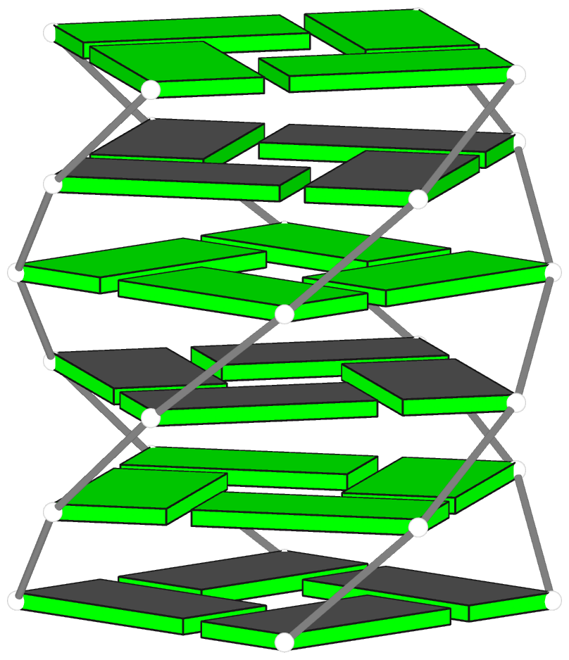
Theoretical models of G-quadruplexes, created using DSSR Pro.

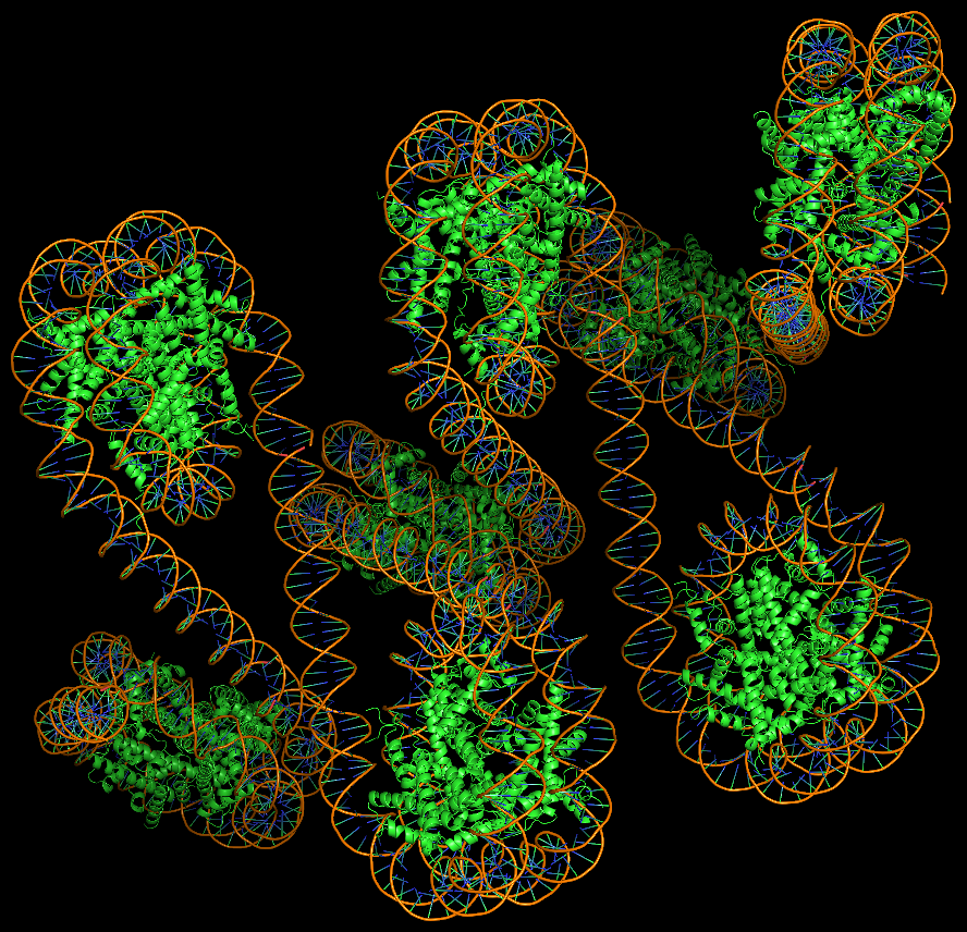
Template-based modeling of DNA-protein complexes using DSSR Pro.
Here are two chromatin-like models using PDB entry 4xzq as the template.


Circular DNA duplexes modeled using DSSR Pro.
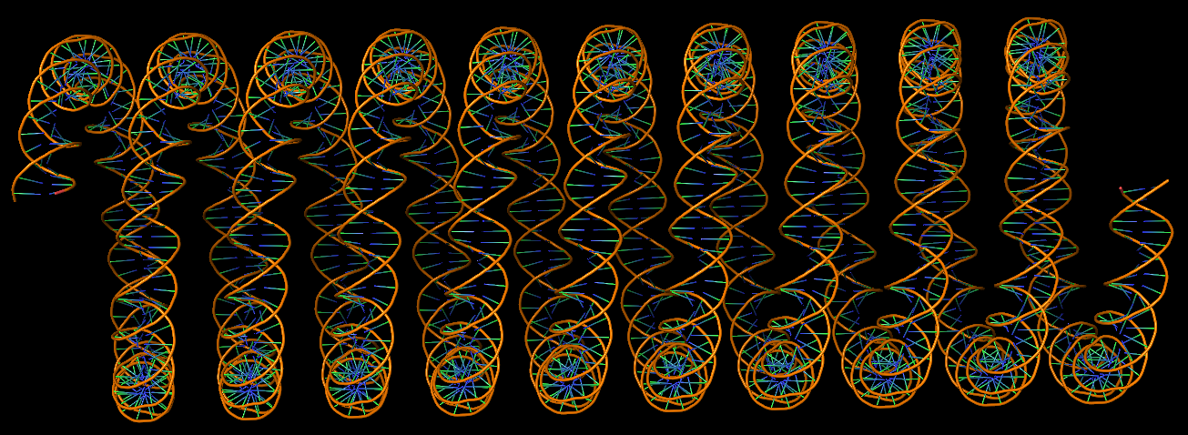
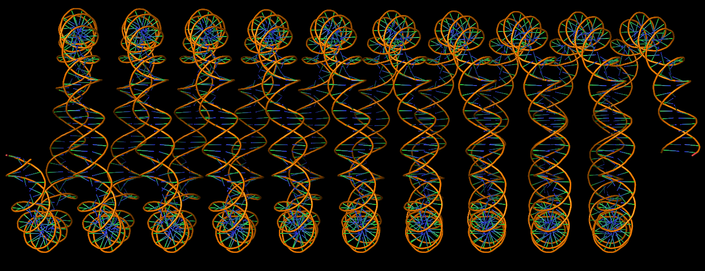
DNA super helices modeled using DSSR Pro.

Innovative cartoon-block schematics enabled by the DSSR-PyMOL integration for six representative PDB entries. Watson-Crick pairs are shown as long blocks with minor-groove edges in black (A, B), G-tetrads represented as square blocks and the metal ion as sphere ©, the ligand rendered as balls-and-sticks (D), and proteins depicted as purple cartoons (E, F). Color code for base blocks: A, red; C, yellow; G, green; T, blue; U, cyan; G-tetrad, green; WC-pairs, per base in the leading strand. Visit http://skmatic.x3dna.org.
Recommended in Faculty Opinions: “simple and effective”, “Good for Teaching”.
Employed by the NDB to create cover images of the RNA Journal.
DSSR (Dissecting the Spatial Structure of RNA) is an integrated software tool for the analysis/annotation, model building, and schematic visualization of 3D nucleic acid structures (see the figures below and the video overview). It is built upon the well-known, tested, and trusted 3DNA suite of programs. DSSR has been made possible by the developer’s extensive user-support experience, detail-oriented software engineering skills, and expert domain knowledge accumulated over two decades. It streamlines tasks in RNA/DNA structural bioinformatics, and outperforms its ‘competitors’ by far in terms of functionality, usability, and support.
DSSR has been widely cited in scientific literature, and adopted into numerous structural bioinformatics resources. Notably, the DSSR-Jmol and DSSR-PyMOL integrations bring unparalleled search capabilities (e.g., ‘select junctions’ for all multi-branch loops) and innovative visualization styles into 3D nucleic acid structures.
3DNA is a versatile, integrated software system for the analysis, rebuilding and visualization of three-dimensional nucleic-acid-containing structures, including their complexes with proteins and other ligands. At its core, the software uses a simple matrix-based scheme for calculating a complete set of rigid-body parameters that characterize the spatial relationship of the base pairs in DNA and RNA structures. In 3DNA, structural analysis and model rebuilding are the two sides of the same coin: the description of structure is geometrically straightforward and the computation of parameters is mathematically rigorous, allowing for exact rebuilding of a molecular structure based on the derived parameters. Other unique features of 3DNA include: (1) the automatic detection of all possible base pairs, higher-order base associations and helical fragments, which makes analyzing nucleic-acid structures straightforward; (2) a comprehensive collection of 55 fiber models of regular DNA and RNA helices in various polymorphic forms and stoichiometries; (3) generation of base rectangular block schematic presentations highly effective in revealing the key features of small- to medium-sized nucleic-acid structures; (4) in silico base mutation with the sugar-phosphate backbone untouched and the original base reference frame conserved, handy for theoretical studies of DNA-protein interactions; and (5) DSSR for a comprehensive characterization of RNA (secondary) structures from three-dimensional coordinates.
3DNA is written in strict ANSI C computer language, with connecting Ruby scripts. The software package consists of over two-dozen executable programs that can be run directly from the command line in a Unix/Linux-like environment (including Mac OS X, and MinGW/MSYS and Cygwin on Windows). The software has been designed following the Unix philosophy: “Write programs that do one thing and do it well. Write programs to work together.” Each 3DNA component program aims to solve a specific set of closely related problems practically: robust and efficient, getting its job done and then out of the way. Once the user is familiar with the package, it is straightforward to combine the various pieces and other command-line-driven (or capable) tools in a script to automate commonly repeated tasks. Moreover, w3DNA provides a convenient web-interface to commonly used functionality of 3DNA, making the tool accessible to bench scientists, novices non-Linux/Unix users and for educational purposes.
3DNA originated in the SCHNAaP and SCHNArP complementary pair of programs to compute DNA rigid-body parameters and to reconstruct structures from those parameters. Our efforts to resolve the discrepancies among nucleic-acid conformational analysis programs and the consequent definition of the standard base reference frame by the structural biology community prompted us to take advantage of various features in the earlier programs and to adopt the standard frame in 3DNA. The 3DNA software was first made available on the Internet in late 1999, v1.5 was released in late 2002, and then v2.0 in 2008 to accompany the Nature Protocols paper. 3DNA is checked against all NDB entries before each major release to ensure that it works in real world applications. Over the years, we have taken each and every 3DNA-related question from a wide spectrum of user community as an opportunity to improve the functionality of the software. We strive to respond to users as quickly and concretely as possible, often with a step-by-step recipe, until an issue is resolved. This process has helped us to refine and improve the software and has prompted us to add new functionality.
Today, 3DNA has become a prominent structural bioinformatics tool, and is widely used in the scientific community. Overall, 3DNA has received near 900 citations in articles published in ~100 peer-reviewed biology, chemistry and material sciences journals. Broadly speaking, 3DNA’s applications fall into the following three categories: (1) as a standard method for nucleic acid structural analysis; (2) integrated into various structural bioinformatics resources, including the NDB and PDB; (3) enabling new scientific discoveries — 3DNA’s rigorous and reversible engine for the analysis/rebuilding of nucleic acid structures and its efficient and robust implementation in a single software package allow for new hypotheses to be formulated and validated against a large number of structures.
3DNA was initially created by Dr. Xiang-Jun Lu during 1999 to 2002 while working as a post-doctoral research associate in Dr. Wilma Olson’s laboratory at Rutgers — the State University of New Jersey. Thereafter, Dr. Lu — in collaboration with Dr. Olson — had continued to maintain and support 3DNA in his spare time as a sideline project. As of September 2011, 3DNA has been supported by an NIH R01 grant (GM096889), titled “Continued Development and Maintenance of the 3DNA Suite of Programs.” As PI of the funded project, Dr. Lu is now dedicated to pushing 3DNA to the next level to better serve the ever-changing needs of an ever-growing user community. We are working on a new release (currently in beta test) of 3DNA v2.1, which contains refinements/bug-fixes of v2.0, and significant new features.
The following links point to tools that are relevant to 3DNA.
- Curves+ — an updated version of the well-known Curves program, and it conforms to the standard base reference frame.
- 3D-DART — 3DNA-Driven DNA Analysis and Rebuilding Tool. Another web-interface to commonly used 3DNA functionality.
- do_x3dna — “do_x3dna has been developed for analysis of the DNA/RNA dynamics during the molecular dynamics simulations. It uses the 3DNA package to calculate several structural descriptors of DNA/RNA from the GROMACS MD trajectory. It executes 3DNA tools to calculate these descriptors and subsequently, extracts these output and saves into external output files as a function of time.”
- SwS — a Solvation web Service for Nucleic Acids where 3DNA plays a role.
- Raster3D — a set of tools for generating high-quality raster images of proteins or other molecules.
- MolScript — a program for displaying molecular 3D structures, such as proteins, in both schematic and detailed representations.
- Jmol — an open-source Java viewer for chemical structures in 3D with features for chemicals, crystals, materials, and biomolecules.
- PyMOL — a user-sponsored molecular visualization system on an open-source foundation.
- ImageMagick — a software suite to create, edit, compose, or convert bitmap images.
- NDB — Nucleic acids database.
- SBGrid — Excellent services for structural biology laboratories as well software developers.
We always welcome user’s feedback in order to improve 3DNA to serve the community better. If you have any 3DNA-related questions, please do not hesitate to post them on the 3DNA forum — that’s what it’s been created for. I am monitoring the forum on a regular basis, and strive to respond to each and every question posted there quickly and concretely.
You can reach me via email xiangjun@x3dna.org, and find details of my research profile at Google scholar. Wherever practical, I’m open to new collaborative projects of common interest. Particularly, I look forward to cooperating with fellow scientists who are responsive and preferably can communicate in technical details.
Over the years, 3DNA had benefited greatly from interactions with the NDB project led by Professor Helen Berman. Zukang Feng at the PDB/NDB, A. R. Srinivarsan, Andrew Colasanti, Guofei Zheng, Mauricio Esguerra and other members of the Olson laboratory, Surjit Dixit (Wesleyan University), Pascal Auffinger (IBMC/CNRS, France), Ben Eisenbraun (SBGrid Consortium, Harvard Medical School), and numerous users have helped in making 3DNA a better tool to serve the scientific community.
The 3DNA software, its homepage and forum have been created and maintained by Xiang-Jun Lu. Unless specified explicitly otherwise, all posts at x3dna.org are written by Xiang-Jun Lu. The favicon and logo of the homepage and the forum were designed by Jessalyn Lu. The three 3DNA-related services — w3DNA, 3DNALandscapes and BPS — are supported by the Olson laboratory at Rutgers University.
The 3DNA project is supported by the NIH grant R01GM096889.
The v2.1 release of 3DNA, currently in beta, contains many refinements of existing C programs, a complete migration from Perl scripts to Ruby, and additions of several significant new programs. All know bugs in v2.0 have been fixed. Highlights include:
- Added mutate_bases to perform in silico base mutations in nucleic-acid-containing structures (DNA, RNA, and their complexes with ligands and proteins). The program has two key and unique features: (1) the sugar-phosphate backbone conformation is untouched; (2) the base reference frame (position and orientation) is reserved, i.e., the mutated structure shares the same base-pair/step parameters as those of the native structure.
- Added
x3dna_ensemble, a Ruby script to automate the processing of an NMR structure ensemble or MD trajectories in MODEL/ENDMDL delineated PDB format. It has sub-commands analyze, extract, reorient, and block_iamge. To add: convert to transform Amber, Gromacs or CHARMM trajectories.
- Enhanced
find_pair with -c+ option for generating input to Curves+.
- Expanded
fiber with the -s option for generating single stranded structures; the -seq option for specifying base sequence directly on the command line; and the -r option for generating RNA structures (single or double stranded) of arbitrary ACGU sequences.
- Updated the ‘baselist.dat’ file to incorporate all types of NDB/PDB nucleotides as of February 15, 2015; refined
find_pair/analyze/mutate_bases etc to automatically detect and assign of modified bases.
- Renamed Atomic_a.pdb and Atomic.a.pdb etc for modified bases to account for Mac OS X filesystem case sensitivity issue; Copied all Perl scripts to a new directory
perl_scripts/.
- 3DNA now generates PDB files that are compliant with PDB format v3.x, and also has option to allow for three-letter nucleotide names, thus directly compatible with PdbViewer and HADDock. An option is provided to convert 3DNA-generated base rectangular blocks in Alchemy to the more widely accepted MDL molfile format (e.g. by PyMOL).
Recently, I (together with Drs. Wilma Olson and Harmen Bussemaker – a team with a unique combination of complementary expertise) published a new article in Nucleic Acids Research (NAR): The RNA backbone plays a crucial role in mediating the intrinsic stability of the GpU dinucleotide platform and the GpUpA/GpA mini duplex. The key findings of this work are summarized in the abstract:
The side-by-side interactions of nucleobases contribute to the organization of RNA, forming the planar building blocks of helices and mediating chain folding. Dinucleotide platforms, formed by side-by-side pairing of adjacent bases, frequently anchor helices against loops. Surprisingly, GpU steps account for over half of the dinucleotide platforms observed in RNA-containing structures. Why GpU should stand out from other dinucleotides in this respect is not clear from the single well-characterized H-bond found between the guanine N2 and the uracil O4 groups. Here, we describe how an RNA-specific H-bond between O2’(G) and O2P(U) adds to the stability of the GpU platform. Moreover, we show how this pair of oxygen atoms forms an out-of-plane backbone ‘edge’ that is specifically recognized by a non-adjacent guanine in over 90% of the cases, leading to the formation of an asymmetric miniduplex consisting of ‘complementary’ GpUpA and GpA subunits. Together, these five nucleotides constitute the conserved core of the well-known loop-E motif. The backbone-mediated intrinsic stabilities of the GpU dinucleotide platform and the GpUpA/GpA miniduplex plausibly underlie observed evolutionary constraints on base identity. We propose that they may also provide a reason for the extreme conservation of GpU observed at most 5’-splice sites.
As a nice surprise, this publication was selected by NAR as a featured article! According to the NAR website:
Featured Articles highlight the best papers published in NAR. These articles are chosen by the Executive Editors on the recommendation of Editorial Board Members and Referees. They represent the top 5% of papers in terms of originality, significance and scientific excellence.
I feel very gratified with the “extra” recognition. From my own perspective, I can easily rank this paper as the top one in my publication list: from the very beginning, I has been struck by the simplicity and elegance of the GpU story. Hopefully, time will verify the validity of this scientific contribution.
Behind the hood, though, there is a long, complex (sometimes perplexing), yet interesting story associated with this work. Here is how it got started. While writing the 3DNA 2008 Nature Protocols (NP) paper, I selected the (previously undocumented) ‘-p’ option of find_pair to showcase its capability to identify higher-order base associations, using the large ribosomal subunit (1jj2) as an example. I noticed the unexpected O2’(G)⋅⋅⋅O2P H-bond within the GpU dinucleotide platform in a pentaplet (Figure A below). I was/am well aware of Leontis-Westholf’s pioneering work on Geometric nomenclature and classification of RNA base pairs which involves three distinct edges – the Watson-Crick edge, the Hoogsteen edge, and the Sugar edge, yet without taking into consideration of possible sugar-phosphate backbone interactions (Figure B below). So I decided to double-check, just to be sure that the H-bond was not spurious due to defects in the H-bond detecting scheme of find_pair, and the finding was very surprising.

The following section was re-added into the 3DNA NP paper in the very last revision:
It is also worth noting that the G1971–U1972 platform is stabilized not only by the well-characterized G(N2)⋅⋅⋅U(O4) H-bond interaction, but also by a little-noticed G(O2’)⋅⋅⋅U(O2P) sugar-phosphate backbone interaction (Fig. 6a). Examination of the 50S large ribosomal unit (1JJ2) alone reveals ten such double H-bonded G–U platforms, far more occurrences than those registered by any other dinucleotide platform (including A–A) in this structure. Apparently, the G–U platform is more stable than other platforms with only a single base–base H-bond interaction. We are currently investigating this overrepresented G–U dinucleotide platform in other RNA structures. (p.1226)
See also Is the O2’(G)…O2P H-bond in GpU platforms real?
Structural analysis of nucleic acids used to be a rather tedious process, especially for irregular, complicated RNA structures and nucleic-acid/protein complexes [e.g., the large ribosomal subunit of H. marismortui (1jj2)]. Without valid base-pairing information arranged properly in a duplex fragment as input, analysis programs such as Curves+ and analyze/cehs in 3DNA would produce meaningless results. The program find_pair in 3DNA was originally created to solve this specific problem, i.e., to generate an input file to 3DNA analysis routines directly from a nucleic-acid containing structure in PDB format. It is what makes nucleic acids structural analysis a routine process — running through thousands of structures from NDB/PDB can be fully automated.
Overall, find_pair has more than fulfilled the goal of its initial design (as stated above). Over the past few years, its functionality has been expanded and continuously refined (kaizen 改善), making find_pair itself a full-featured application. Now, it is efficient, robust, and its simple command line interface allows for easy integration with other bioinformatics tools. Properly acknowledged or otherwise, find_pair has served (at least) as one of the key components in many other applications (RNAView, BPS, SwS, ARTS, to name just a few). Indeed, find_pair is by far the single program in 3DNA that has received the most questions (as evident from the 3DNA forum).
While I still have to write a method paper to describe the underlying algorithms of find_pair in detail — i.e., for identifying nucleotides, H-bonds, base pairs, high-order base associations, and double helical regions — the basic idea is intuitive and very easy to understand: as summarized in our recent GpU paper”, find_pair is purely geometric based (with user adjustable parameters) and allows for the identification of canonical Watson–Crick as well as non-canonical base pairs, made up of normal or modified bases, regardless of tautomeric or protonation state. For example, in the GpU paper”, we chose the following set of stringent parameters to ensure that the geometry of each identified base pair is nearly planar and supports at least one inter-base H-bond: (i) a vertical distance (stagger) between base planes ≤ 1.5 Å; (ii) an angle between base normal vectors ≤ 30°; and (iii) a pair of nitrogen and/or oxygen base atoms at a distance ≤ 3.3 Å. Other criteria (documented or otherwise), such as the distance between the origins of the two standard base reference frames, are just filters to speed up the calculations.
In a nutshell, find_pair has the following two core functionalities:
- The default is to generate input to the analysis routines in 3DNA (
analyze/cehs) for double helices. However, there are many more job to perform under the hood than just identifying base pairs: the base pairs must be in proper sequential order, and each strand must be in 5’ to 3’ direction, for the calculated step parameters (twist, roll etc) to make sense. Moreover, with the “-c” option, one gets an input file to Curves (but not Curves+, yet); with the “-s” or “-1” option, find_pair treats the whole structure as one single strand, and is useful for getting all backbone torsion angles.
- Detect all base pairs (regardless of double helical regions) and higher-oder (3+) base associations with the “-p” option. This feature (in its preliminary form) was there starting from at least v1.5, which was released at the end of 2002 (just before I left Rutgers), but it was intentionally undocumented. The source code of
find_pair (as part of 3DNA) was tested and shared within Rutgers (NDB and Dr. Olson’s laboratory) before any 3DNA paper was published, and served as the basis for several other projects. We also offered 3DNA (with source code) to a few RNA experts for comments; but we received either no responses or politely-worded negative ones. Things did not work out as (what I thought) they should have been, but that’s life and I have learned my lessons. The “-p” option was first explicitly mentioned in the 3DNA 2008 Nature Protocols paper, to illustrate how to identify the two pentaplets in the large ribosomal subunit of H. marismortui (1jj2).
It is interesting to mention the two papers I’ve recently come across: the first is on DNA-protein interactions and the second on RNA base-pairing, where new algorithms were developed to detect base pairs and their performances were compared with find_pair. In each of the two cases, it was claimed that find_pair missed certain pairs where the new methods succeeded. As it turned out, however, in the first case, simply relaxing find_pair’s default H-bond distance cut-off 4.0 Å to 4.5 Å, as used by the authors, virtually all the missing pairs were recovered. In the second case, the “-p” option, which should have been, was simply not specified.
After nearly a decade of extensive real-world applications and refinements, it is safe to say that find_pair is now a versatile and practical tool for nucleic acids structure analysis. Of course, I will continue to support and further refine find_pair as I see fit. Once in a while, I just cannot stop but to think that find_pair is to nucleic acids what DSSP is to proteins: simple and elegant. As more people become aware of its existence, I would expect find_pair to gain even more widespread usage, especially in RNA-structure related research areas.
While browsing Nucleic Acids Research recently, I noticed the paper titled Conformational analysis of nucleic acids revisited: Curves+ by Dr. Lavery et al. I read it through carefully during the weekend and played around with the software. Overall, I was fairly impressed, and also happy to see that “It [Curves+] adopts the generally accepted reference frame for nucleic acid bases and no longer shows any significant difference with analysis programs such as 3DNA for intra- or inter-base pair parameters.”
Anyone who has ever worked on nucleic acid structures (especially DNA) should be familiar with Curves, an analysis program that has been widely used over the past twenty years. Only in recent years has 3DNA become popular. By and large, though, it is my opinion that 3DNA and Curves are constructive competitors in nucleic acid structure analysis with complementary functionality. As I put it six years ago, before the 13th Conversation at Albany: “Curves has special features that 3DNA does not want to repeat/compete (e.g. global parameters, groove dimension parameters). Nevertheless, we provide an option in a 3DNA utility program (find_pair) to generate input to Curves directly from a PDB data file” on June 6, 2003, and emphasized again on June 09, 2003: “We also see Curves unique in defining global parameters, bending analysis and groove dimensions.” 3DNA’s real strength, as demonstrated in our 2008 Nature Protocols paper, lies in its integrated approach that combines nucleic acid structure analysis, rebuilding, and visualization into a single software package (see image below).

Now the nucleic acid structure community is blessed with the new Curves+, which “is algorithmically simpler and computationally much faster than the earlier Curves approach”, yet still provides its ‘hallmark’ curvilinear axis and “a full analysis of groove widths and depths”. When I read the text, I especially liked the INTRODUCTION section, which provides a nice summary of relevant background information on nucleic acid conformational analysis. An important feature of Curves+ is its integration of the analysis of molecular dynamics trajectories. In contrast, 3DNA lacks direct support in this area (even though I know of such applications from questions posted on the 3DNA forum), mostly due to the fact that I am not an ‘energetic’ person. Of special note is a policy-related advantage Curves+ has over 3DNA: Curves+ is distributed freely, and with source code available. On the other hand, due to Rutgers’ license constraints and various other (undocumented) reasons, 3DNA users are still having difficulty in accessing 3DNA v2.0 I compiled several months ago!
It is worth noting that the major differences in slide (+0.47 Å) and x-displacement (+0.77 Å) in Curves+ vs the old Curves (~0.5 Å and ~0.8 Å, respectively) are nearly exactly those uncovered a decade ago in Resolving the discrepancies among nucleic acid conformational analyses [Lu and Olson (1999), J. Mol. Biol., 285(4), 1563-75]:
Except for Curves, which defines the local frame in terms of the canonical B-DNA fiber structure (Leslie et al., 1980), the base origins are roughly coincident in the different schemes, but are significantly displaced (~0.8 Å along the positive x-axis) from the Curves reference. As illustrated below, this offset gives rise to systematic discrepancies of ~0.5 Å in slide and ~0.8 Å in global x-displacement in Curves compared with other programs, and also contributes to differences in rise at kinked steps. (p. 1566)
Please note that Curves+ has introduced new name list variables — most notably, lib= — and other subtle format changes, thus rendering the find_pair generated input files (with option ‘-c’) no longer valid. However, it would be easy to manually edit the input file to make it work for Curves+, since the most significant part — i.e., specifying paired nucleotides — does not change. Given time and upon user request, however, I would consider to write a new script to automate the process.
Overall, it is to the user community’s advantage to have both 3DNA and Curves+ or a choice between the two programs, and I am more than willing to build a bridge between them to make users’ lives easier.


")
")
 in cartoon-block representation")
 RNA (4jrd)")
 with base blocks")
 with WC base-pair blocks")
 of the C-G pair that closes the GUAA tetraloop facing the viewer")
 -- base blocks in outline")
")
")


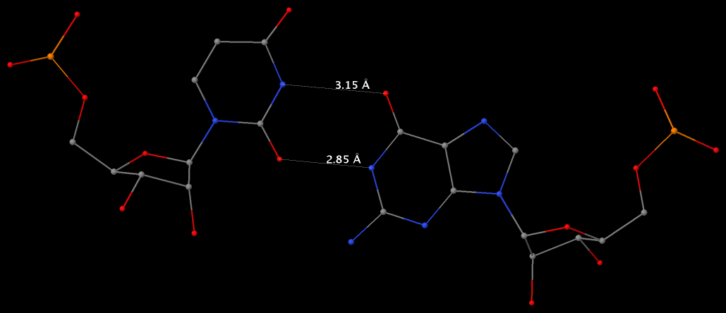
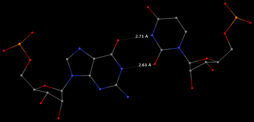
 with a designer antibiotic (2f4u).")
.")
.")
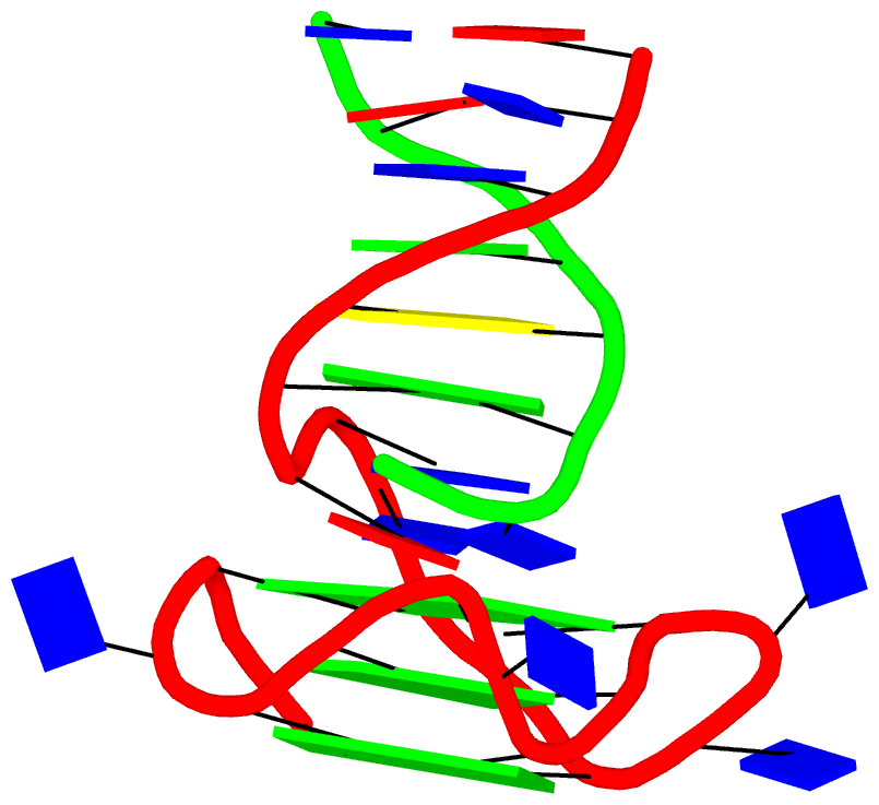
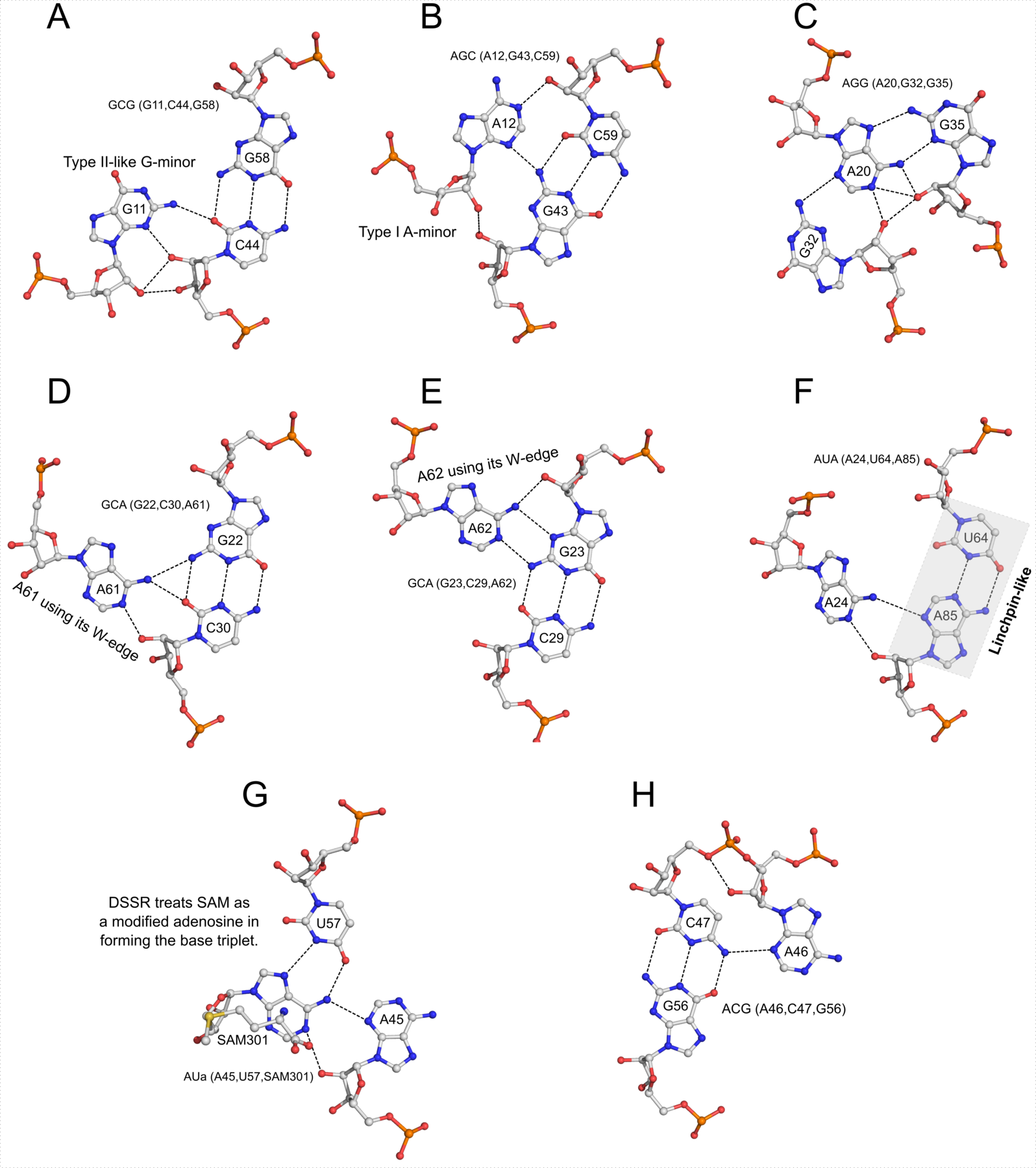