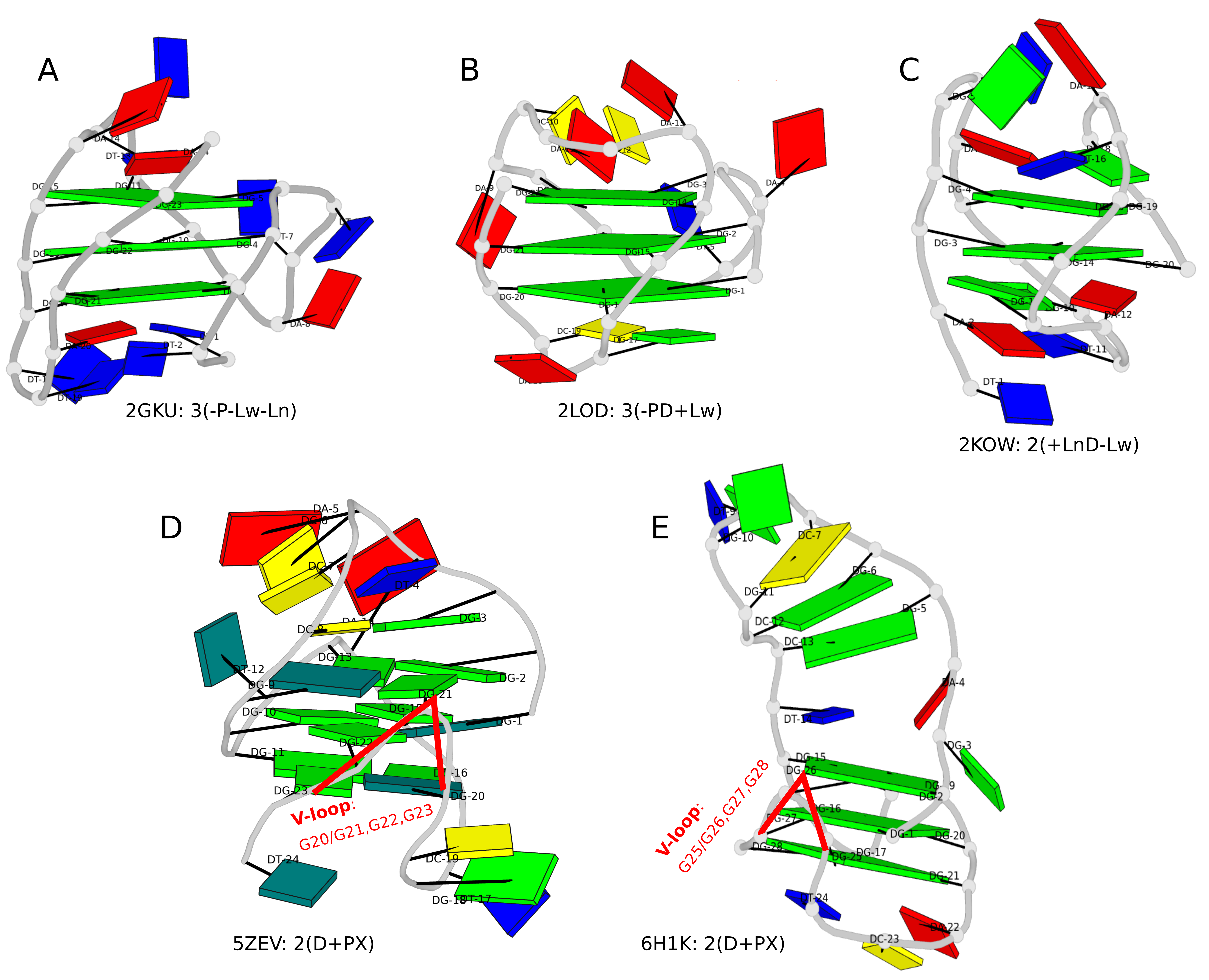
Over the past couple of months, I’ve further enhanced the DSSR-derived structural features for Q-quadruplexes (G4). One was the implementation of the single descriptor of intramolecular canonical G4 structures with three connecting loops recently proposed by Dvorkin et al. The descriptor contains the number of guanines in the G4 stem, the type and relative direction of loops linking G-tracts of the stem, and the groove-widths associated with lateral loops. For example, PDB entry 2GKU (see the DSSR-enabled PyMOL schematic image below, Fig. 1A) has the following DSSR output.

List of 1 G4-stem
  Note: a G4-stem is defined as a G4-helix with backbone connectivity.
        Bulges are also allowed along each of the four strands.
  stem#1[#1] layers=3 INTRA-molecular loops=3 descriptor=3(-P-Lw-Ln) note=hybrid-1(3+1) UUDU anti-parallel
   1  glyco-bond=ss-s groove=-wn- mm(<>,outward)  area=14.24 rise=3.58 twist=16.8  nts=4 GGGG A.DG3,A.DG9,A.DG17,A.DG21
   2  glyco-bond=--s- groove=-wn- pm(>>,forward)  area=13.12 rise=3.71 twist=25.9  nts=4 GGGG A.DG4,A.DG10,A.DG16,A.DG22
   3  glyco-bond=--s- groove=-wn-                                                  nts=4 GGGG A.DG5,A.DG11,A.DG15,A.DG23
    strand#1  U DNA glyco-bond=s-- nts=3 GGG A.DG3,A.DG4,A.DG5
    strand#2  U DNA glyco-bond=s-- nts=3 GGG A.DG9,A.DG10,A.DG11
    strand#3  D DNA glyco-bond=-ss nts=3 GGG A.DG17,A.DG16,A.DG15
    strand#4  U DNA glyco-bond=s-- nts=3 GGG A.DG21,A.DG22,A.DG23
    loop#1 type=propeller strands=[#1,#2] nts=3 TTA A.DT6,A.DT7,A.DA8
    loop#2 type=lateral   strands=[#2,#3] nts=3 TTA A.DT12,A.DT13,A.DA14
    loop#3 type=lateral   strands=[#3,#4] nts=3 TTA A.DT18,A.DT19,A.DA20

The descriptor=3(-P-Lw-Ln) means that the G4 structure has three layers of G-tetrads, connected via three loops: the first is the Propeller loop in anti-clockwise (negative) direction, then the Lateral loop passing a wide groove anti-clockwise, and finally another Lateral loop passing a narrow groove, also anti-clockwise. The DSSR symbols follow those of Dvorkin et al. but with capital letters L, P, and D for lateral, propeller, and diagonal loops instead of lower case letters (l, p, d) to avoid using subscript for groove-width info. So the 2GKU descriptor 3(-P-Lw-Ln) from DSSR corresponds to 3(-p-l_w-l_n) of Dvorkin et al.

The DSSR-enabled, PyMOL-rendered, block image in Fig. 1A makes the three G-tetrad layers (squared green blocks) immediately obvious. Other base identities and stacking interactions also become clear — for example, the A24 (in red) stacks on the top G-tetrad, and T1-A20 pair stacks with the bottom G-tetrad.

Two other PDB entries (2LOD and 2KOW) are illustrated in Fig. 1B and Fig. 1C. They have different topologies than 2GKU (Fig. 1A). DSSR is able to characterize all of them consistently.

Figure 1. DSSR-enabled, PyMOL-rendered, block images of five G-quadruplexes. A in red, C in yellow, G (and G-tetrad) in green, and T in blue.

Another G4-related new feature in DSSR is the detection of V-shaped loops in noncanonical G4 structures where one of the four G-G columns (strands) that link adjacent G-tetrads is broken. Two of recent PDB examples with V-loops are shown in Fig. 1D (5ZEV) and Fig. 1E (6H1K). An excerpt of DSSR output for the PDB entry 6H1K is shown below.

List of 1 G4-helix
  Note: a G4-helix is defined by stacking interactions of G4-tetrads, regardless
        of backbone connectivity, and may contain more than one G4-stem.
  helix#1[1] stems=[#1] layers=3 INTRA-molecular
   1  glyco-bond=-sss groove=w--n mm(<>,outward)  area=12.76 rise=3.47 twist=18.2  nts=4 GGGG A.DG2,A.DG19,A.DG15,A.DG26
   2  glyco-bond=s--- groove=w--n pm(>>,forward)  area=12.84 rise=3.07 twist=33.4  nts=4 GGGG A.DG1,A.DG20,A.DG16,A.DG27
   3  glyco-bond=s--- groove=w--n                                                  nts=4 GGGG A.DG25,A.DG21,A.DG17,A.DG28
    strand#1 DNA glyco-bond=-ss nts=3 GGG A.DG2,A.DG1,A.DG25
    strand#2 DNA glyco-bond=s-- nts=3 GGG A.DG19,A.DG20,A.DG21
    strand#3 DNA glyco-bond=s-- nts=3 GGG A.DG15,A.DG16,A.DG17
    strand#4 DNA glyco-bond=s-- nts=3 GGG A.DG26,A.DG27,A.DG28

****************************************************************************
List of 1 G4-stem
  Note: a G4-stem is defined as a G4-helix with backbone connectivity.
        Bulges are also allowed along each of the four strands.
  stem#1[#1] layers=2 INTRA-molecular loops=3 descriptor=2(D+PX) note=UD3(1+3) UDDD anti-parallel
   1  glyco-bond=s--- groove=w--n mm(<>,outward)  area=12.76 rise=3.47 twist=18.2  nts=4 GGGG A.DG1,A.DG20,A.DG16,A.DG27
   2  glyco-bond=-sss groove=w--n                                                  nts=4 GGGG A.DG2,A.DG19,A.DG15,A.DG26
    strand#1  U DNA glyco-bond=s- nts=2 GG A.DG1,A.DG2
    strand#2  D DNA glyco-bond=-s nts=2 GG A.DG20,A.DG19
    strand#3  D DNA glyco-bond=-s nts=2 GG A.DG16,A.DG15
    strand#4  D DNA glyco-bond=-s nts=2 GG A.DG27,A.DG26
    loop#1 type=diagonal  strands=[#1,#3] nts=12 GAGGCGTGGCCT A.DG3,A.DA4,A.DG5,A.DG6,A.DC7,A.DG8,A.DT9,A.DG10,A.DG11,A.DC12,A.DC13,A.DT14
    loop#2 type=propeller strands=[#3,#2] nts=2 GC A.DG17,A.DC18
    loop#3 type=diag-prop strands=[#2,#4] nts=5 GACTG A.DG21,A.DA22,A.DC23,A.DT24,A.DG25

****************************************************************************
List of 2 non-stem G4 loops (INCLUDING the two terminal nts)
   1 type=lateral   helix=#1 nts=5 GACTG A.DG21,A.DA22,A.DC23,A.DT24,A.DG25
   2 type=V-shaped  helix=#1 nts=4 GGGG A.DG25,A.DG26,A.DG27,A.DG28

Note that here a new loop type (diag-prop) and topology description symbol (X) are introduced. In developing DSSR in general, and G4-related features in particular, I’ve always tried to follow conventions widely used by the community. Whereas inconsistency exists, I pick up the ones that are in line with other parts of DSSR. For unique DSSR features lacking outside references, I came up my own nomenclature. When DSSR becomes more widely used, it may serve to standardize G4 nomenclatures.

From early on, the --json and --nmr options in DSSR have provided a convenient means to analyze an ensemble of solution NMR structures in the standard PDB/mmCIF format, as those available from the Protein Data Bank (PDB). The usage is very simple, as shown below for the PDB entry 2lod. The parameters for each model can be easily parsed from the output JSON stream.

A practical example of the DSSR JSON/NMR usage for the analysis of RNA backbone torsion angles can be found on the 3DNA Forum.

While not a practitioner of molecular dynamics (MD) simulations, I’ve regularly followed the relevant literature. I know of the popular tools such as MDanalysis, MDTraj, and CPPTRAJ that are dedicated to analyze trajectories of MD simulations. I understand the subtleties MD may have, and I’m also sure of the unique features DSSR has to offer. By design, I made the DSSR interface to MD straightforward, by simply following commonly-used standard data formats: the MODEL/ENDMDL delineated PDB (or the PDBx/mmCIF) format for input, and JSON for output. Overall, I had expected that DSSR would complement the dedicated tools (e.g., MDanalysis, MDTraj, and CPPTRAJ) for MD analysis.

Over the years, DSSR has gradually gained recognition in the MD field. At a meeting, I once heard of a user complaining that DSSR is too slow for the analysis of millions of frames of MD simulations. Yet, without access to a large MD dataset and direct collaborations from a user, the speed issue could not be pursued further. In my experience, I knew DSSR is fast enough for the analysis of NMR ensembles from the PDB. This situation has completely changed recently, after a user reported on the 3DNA Forum on the slowness of DSSR on MD analysis.

Do you have an idea why the backbone parameter for a nucleic acids are so much faster calculated with do_x3dna than with DSSR? Analyzing a trajectory with 100k frames take for a native structure approx. 2 hours with do_x3dna. A native RNA structure with DSSR will take approx. 10 days (10k frames/day). I need to run DSSR, because my system contains an abasic site.

With the above and follow-up information provided, I was able to fix the DSSR algorithm for parsing MD trajectories, among other things. Now DSSR reads a trajectory sequentially frame-by-frame at constant speed. The same 100K frames takes 36 minutes to finish instead of 10 days, which is an increase of 10*24*60/36=400 times. This 100x speedup was later on verified when I tested DSSR on the 1000-structure trajectory the user supplied.

So as of v1.7.8-2018sep01, DSSR is quick enough for real-world applications on MD analysis. In the releases of DSSR afterwards, I’ve further polished the code and added some new features. All things considered, DSSR is bound to become more relevant in the active MD field in the years to come.

By the way, for those who do not like the --nmr option, --md or --ensemble also works. These three alternatives are equivalent to DSSR internally.

As mentioned in the blog post Integrating DSSR into Jmol and PyMOL,
“The small size, zero configuration, extensive features, and robust performance make DSSR ideal to be integrated into other bioinformatics tools.” In addition to the DSSR-Jmol and DSSR-PyMOL integrations which I initiated and got personally involved, other bioinformatics resources are increasingly taking advantage of what DSSR has to offer. Here are a few examples:

• As of Nov. 7, 2017, DSSR has become the only option for base-pairing annotation in the WebSTAR3D web server for RNA 3D structure alignment. In the 2016 WebSTAR3D publication in Bioinformatics, DSSR was the second choice, as shown in the excerpt below:

Before aligning structures, STAR3D preprocesses PDB files with base-pairing annotation using either MC-Annotate (Gendron et al., 2001; Lemieux and Major, 2002) (for PDB inputs) or DSSR (Lu et al., 2015) (for PDB and mmCIF inputs) and pseudo-knot removal using RemovePseudoknots (Smit et al., 2008).

• In the RNApdbee 2.0 web server for RNA secondary structure annotation, DSSR is the default option for identifying base pairs. See also the corresponding publication in Nucleic Acids Research (2018), titled RNApdbee 2.0: multifunctional tool for RNA structure annotation. In contrast, the first version (published in 2014) of RNApdbee put DSSR as the third option, following RNAView and MC-Annotate. See my blog post titled RNA pseudoknot detection and removal with DSSR, and the excerpts from the 2014 (RNApdbee) and 2018 (RNApdbee 2.0) papers:

2014, RNApdbee: In order to facilitate a more comprehensive study, the webserver integrates the functionality of RNAView, MC-Annotate and 3DNA/DSSR, being the most common tools used for automated identification and classification of RNA base pairs.

2018, RNApdbee 2.0: Base pairs can be identified by 3DNA/DSSR (default) (4), RNAView (5), MC-Annotate (3) or newly added FR3D (15).

• The Universe of RNA Structures (URS) web-interface to the URS database (URSDB) makes extensive use of DSSR. For each analyzed structure (including PDB entries), the DSSR text output file (termed “DSSR-file”) is also available. Impressively, the maintainers of URS are quick with DSSR updates. The current version used by the URS website is DSSR v1.7.4-2018jan30.

Forty years after the yeast phenylalanine tRNA structure was solved, modified nucleotides should no longer be an issue for RNA structural analysis, especially for this classic molecule. Automatic processing of modified nucleotides is just one aspect of DSSR’s substantial set of features. Based on my understanding of the field, more structural bioinformatics resources/tools could benefit from DSSR. Simply put, if one’s project is related to 3D DNA or RNA structures, DSSR may be of certain help. It’s just a timing issue that DSSR would benefit a (much) larger community.

DSSR deliberately makes a distinction between ‘stem’ and ‘helix’, as shown below:

a helix is defined by base-stacking interactions, regardless of bp type and backbone connectivity, and may contain more than one stem.

a stem is defined as a helix consisting of only canonical WC/wobble pairs, with a continuous backbone.

By definition, a helix or stem consists of at least two base-pairs with stacking interactions. Helix is more inclusive and may contain more than one stem. This differentiation between ‘helix’ and ‘stem’ naturally leads to the definition of coaxial stacking, another widely used yet vaguely specified concept.

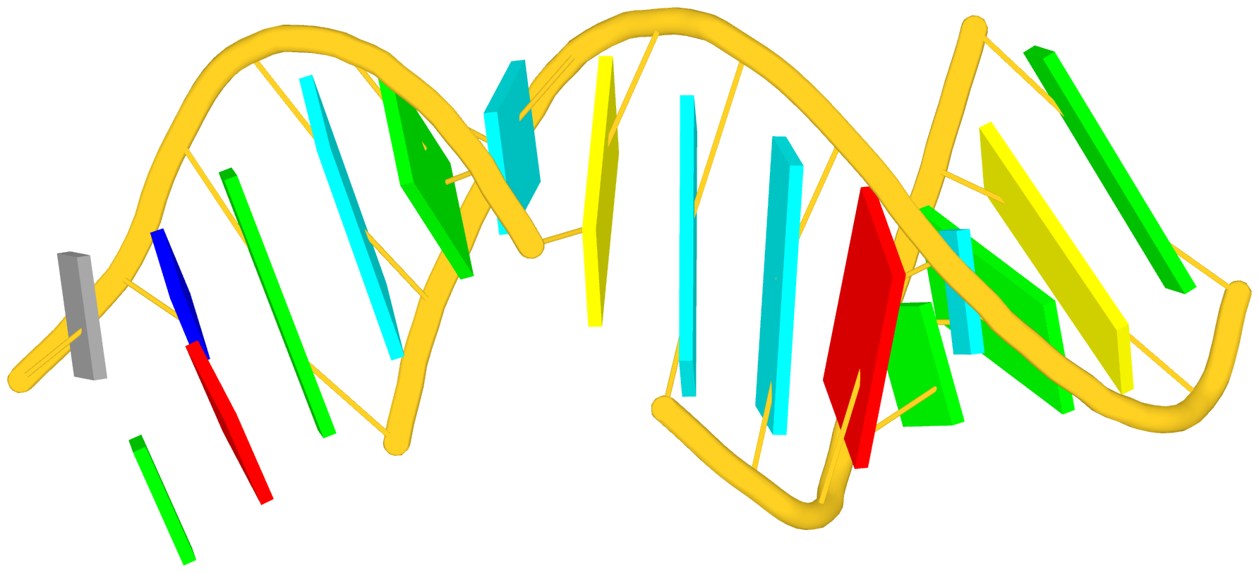
Again, the abstract notion can be best illustrated with a concrete example. In the classic yeast phenylalanine tRNA (PDB id: 1ehz), DSSR identifies that two stems [the acceptor stem (right) and the T stem (left)] are coaxially stacked within one double helix. See the figure below.

In the above schematics cartoon-block representation, each Watson-Crick base pair is rendered as a single, long rectangular block. Base identities of the G–U wobble, and the two non-canonical pairs (left terminal) are illustrated separately, with a larger block size for purines (G and A), and a smaller size for pyrimidines (C, U, and T).

I picked up ‘stem’ as a more specialized duplex because it is widely used in the RNA stem-loop structure, and in describing the four ‘paired regions’ of the classic tRNA cloverleaf secondary structure. On the other hand, ‘helix’ is (to me at least) a more general term, and thus more inclusive. It is worth noting that other terms such as ‘arm’, ‘paired region’, or ‘helix’ etc. have also been used interchangeably in the literature to refer what DSSR designated as ‘stem’.

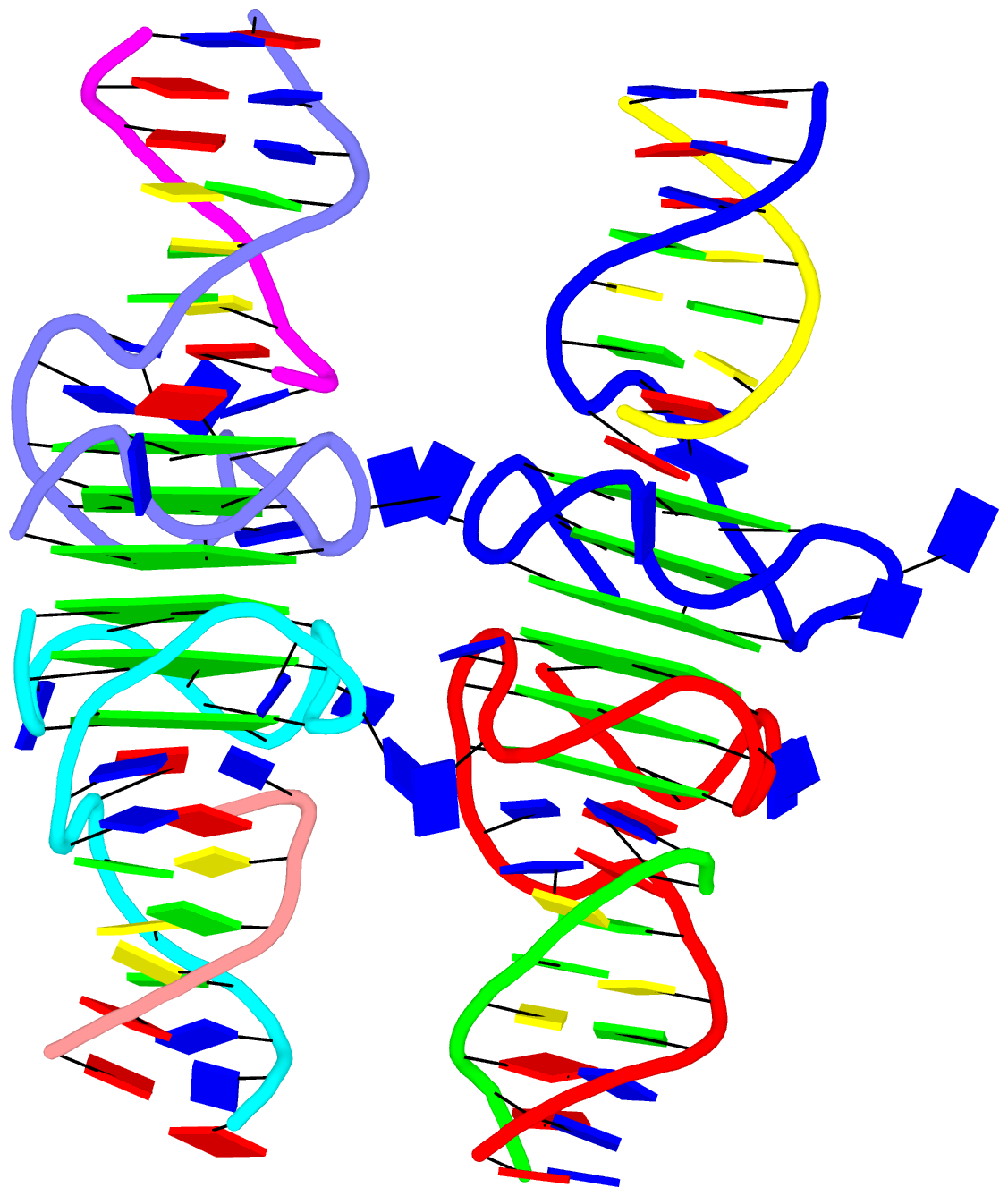
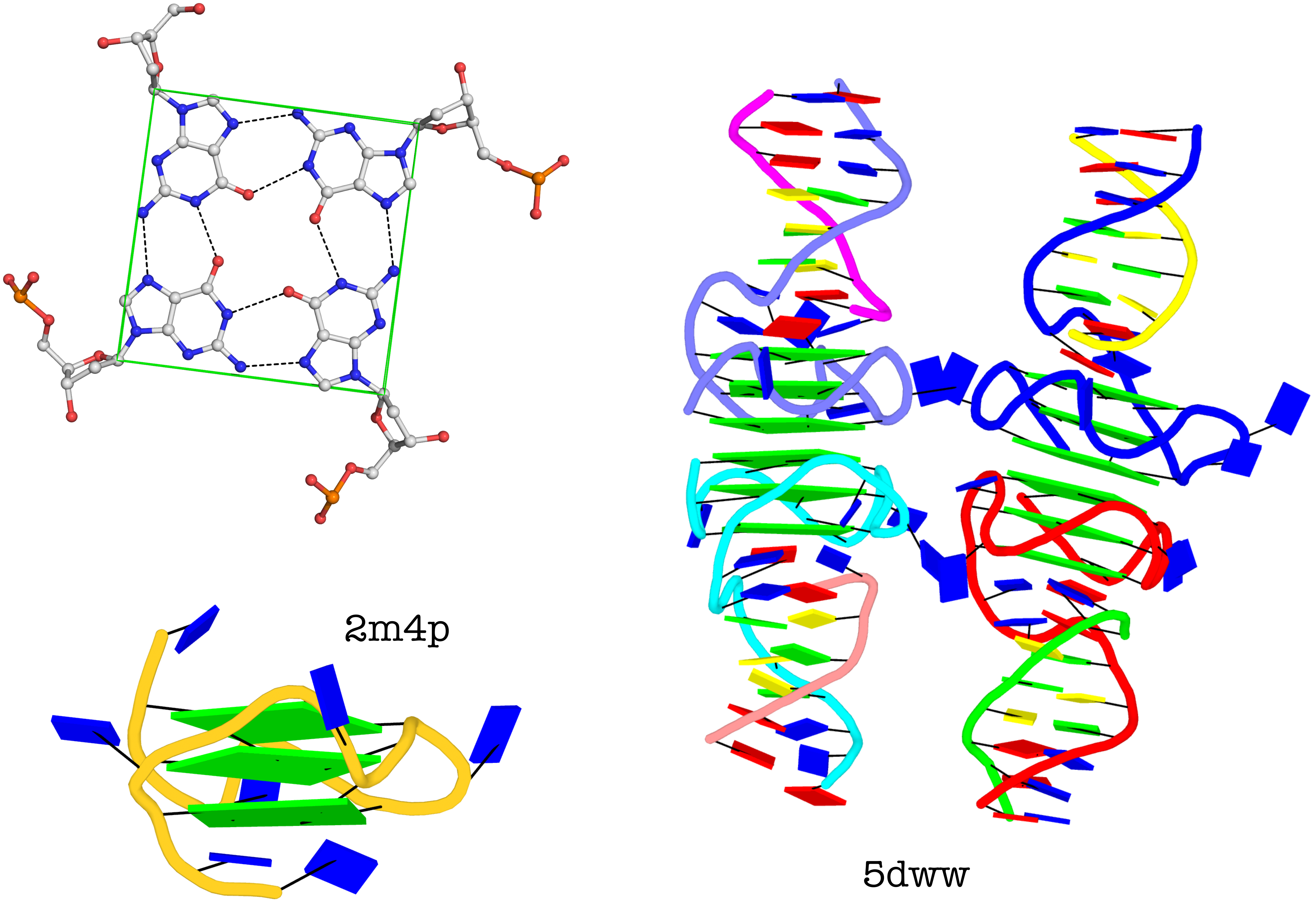
As a side note, the basic algorithm for identifying helixes/stems in DSSR is also applicable for detecting G-quadruplexes. The same idea of ‘helix’ or ‘stem’ also applies here (see figure below for PDB entry: 5dww). Indeed, as of v1.7.0-2017oct19, DSSR contains a new section for the identification and characterization of G-quadruplexes.

DSSR is “an integrated software tool for dissecting the spatial structure of RNA”. It excels in consolidating the diverse pieces together via a coherent framework, readily accessible in a solid software product. DSSR may well serve as a cornerstone in RNA structural bioinformatics and would facilitate communications in the broad areas related to nucleic acids structures.

Among the rich set of RNA structural features derived by DSSR, the section of “List of stacks” apparently has not drawn much attention from the user community. As noted in the DSSR output,

a stack is an ordered list of nucleotides assembled together via base-stacking interactions, regardless of backbone connectivity. Stacking interactions within a stem are not included.

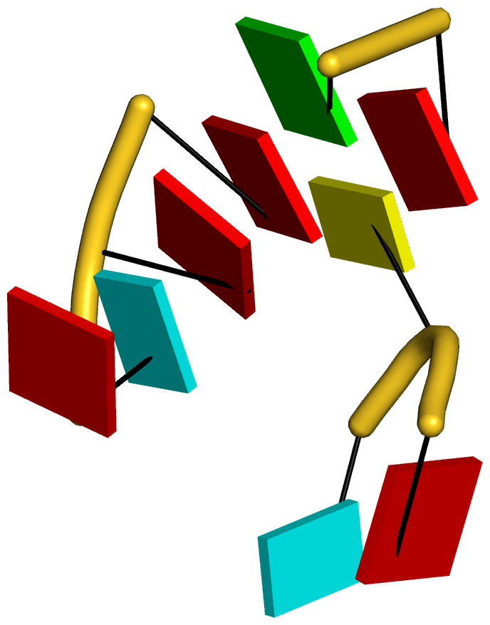
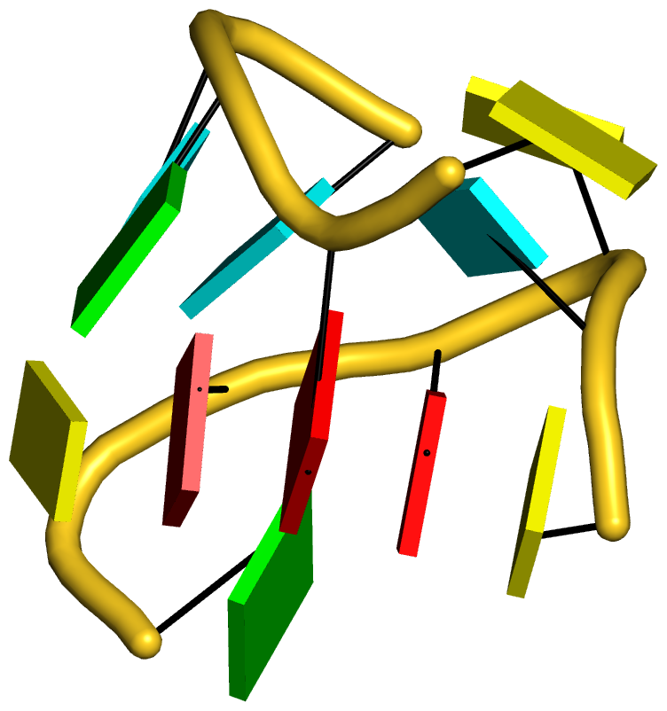
As always, the concept is best illustrated via concrete examples. Shown below are two such base stacks automatically identified by DSSR in the PDB entry 4p5j, the crystal structure of the tRNA-mimic from Turnip Yellow Mosaic Virus (TYMV) which was analyzed in detail in the 2015 DSSR NAR paper

This critical linchpin in the tRNA mimic is stabilized by extensive base-stacking interactions.	The intricate interactions between the D- and T-loops in the tRNA mimic include a five-base stack.

The DSSR-introduced schematic block representation makes the base-stacking interactions immediately obvious. One can even easily discern the identity of bases, given the color-coding convention: A-red; C-yellow; G-green; T-blue; U-cyan. For example, the five stacked bases involved in the interaction of the D- and T-loops are: CAAAC

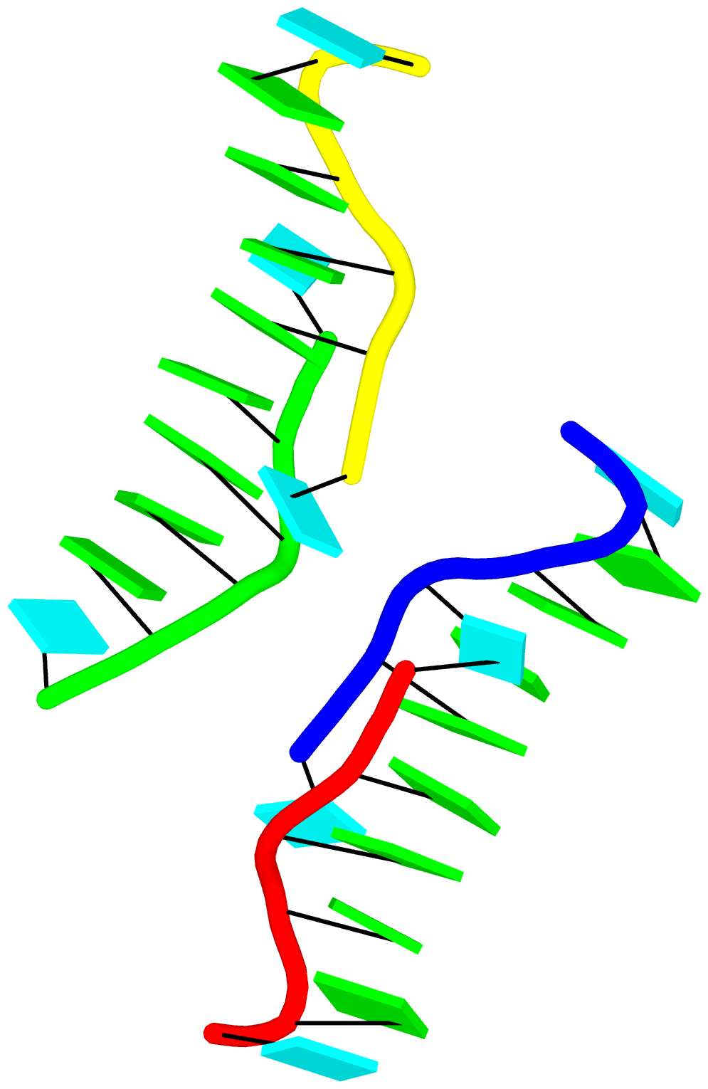
Moreover, longer and more complicate base-stacks can also be auto-detected by DSSR, as shown below for the asymmetric unit of PDB entry 1j8g, the crystal structure of an RNA quadruplex r(UGGGGU)4 at 0.61 Å resolution. Here DSSR identifies two 10-base stacks, each of UGGGGGGGGU (UG8U).

The corresponding DSSR output is as below:

List of 2 stacks
  Note: a stack is an ordered list of nucleotides assembled together via
        base-stacking interactions, regardless of backbone connectivity.
        Stacking interactions within a stem are *not* included.
   1 nts=10 UGGGGGGGGU A.U6,A.G5,A.G4,A.G3,A.G2,C.G22,C.G23,C.G24,C.G25,C.U26
   2 nts=10 UGGGGGGGGU B.U16,B.G15,B.G14,B.G13,B.G12,D.G32,D.G33,D.G34,D.G35,D.U36

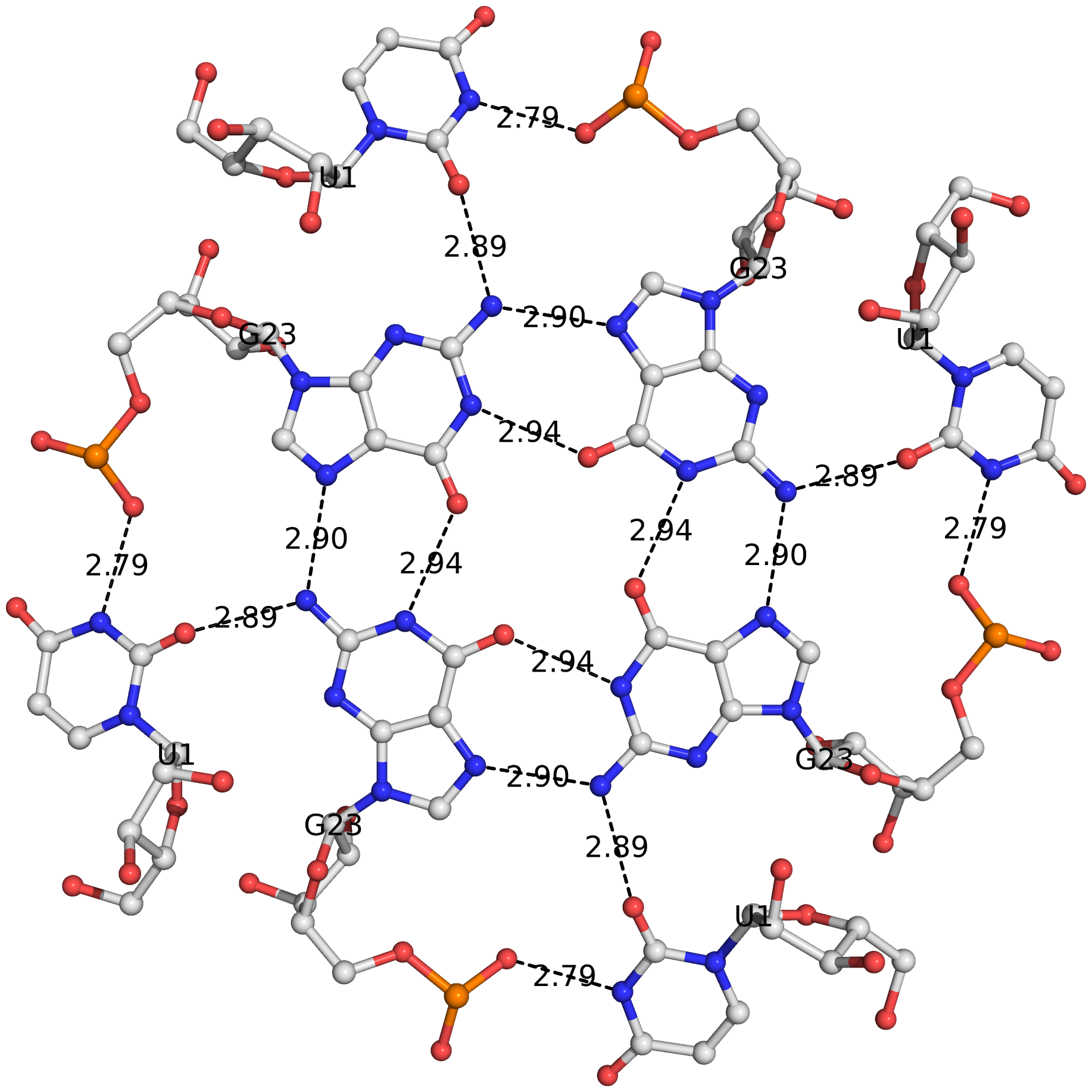
G-quadruplexes (hereafter referred to as G4) are a common type of higher-order DNA and RNA structures formed from G-rich sequences. The building block of G4 is a tetrad of guanines in a cyclic planar alignment, with four G+G pairs (cW+M type, see Figure below). A G4 structure is formed by stacking of G-tetrads and stabilized by cations at the center of the layers. G4 structures are polymorphic: the four strands can be parallel or anti-parallel, and loops connecting them can be of different types: lateral (edgewise), diagonal, or propeller (double-chain reversal). Moreover, G4 structures can be intra- or intermolecular, and even contain bulges.

From its initial releases, DSSR was able to detect G-tetrads, and listed them in a separate section. As of v1.7.0-2017oct19, DSSR has integrated existing features and created a new module to automatically identify and fully characterize G4 structures. The underlying algorithms have been further refined in v1.7.1-2017nov01, which was tested against all nucleic-acid-containing structures in the PDB.

Characterizations of three representative G4 examples (PDB entries 2m4p, 2hy9, and 5hix) are shown below, illustrating salient features (e.g., different types of loops) automatically extracted by DSSR.

2m9p

stem#1[#1] layers=3 INTRA-molecular parallel bulged-strands=1
   1 syn=---- WC-->Major area=8.38  rise=3.64 twist=33.34 nts=4 GGGG A.DG3,A.DG8,A.DG12,A.DG16
   2 syn=---- WC-->Major area=10.73 rise=3.23 twist=32.42 nts=4 GGGG A.DG5,A.DG9,A.DG13,A.DG17
   3 syn=---- WC-->Major                                  nts=4 GGGG A.DG6,A.DG10,A.DG14,A.DG18
    strand#1* +1 DNA syn=--- nts=3 GGG A.DG3,A.DG5,A.DG6 bulged-nts=1 T A.DT4
    strand#2  +1 DNA syn=--- nts=3 GGG A.DG8,A.DG9,A.DG10
    strand#3  +1 DNA syn=--- nts=3 GGG A.DG12,A.DG13,A.DG14
    strand#4  +1 DNA syn=--- nts=3 GGG A.DG16,A.DG17,A.DG18
    loop#1 type=propeller strands=[#1,#2] nts=1 T A.DT7
    loop#2 type=propeller strands=[#2,#3] nts=1 T A.DT11
    loop#3 type=propeller strands=[#3,#4] nts=1 T A.DT15

2hy9

stem#1[#1] layers=3 INTRA-molecular anti-parallel
   1 syn=ss-s Major-->WC area=13.69 rise=3.14 twist=19.08 nts=4 GGGG 1.DG4,1.DG10,1.DG18,1.DG22
   2 syn=--s- WC-->Major area=13.40 rise=3.05 twist=28.05 nts=4 GGGG 1.DG5,1.DG11,1.DG17,1.DG23
   3 syn=--s- WC-->Major                                  nts=4 GGGG 1.DG6,1.DG12,1.DG16,1.DG24
    strand#1  +1 DNA syn=s-- nts=3 GGG 1.DG4,1.DG5,1.DG6
    strand#2  +1 DNA syn=s-- nts=3 GGG 1.DG10,1.DG11,1.DG12
    strand#3  -1 DNA syn=-ss nts=3 GGG 1.DG18,1.DG17,1.DG16
    strand#4  +1 DNA syn=s-- nts=3 GGG 1.DG22,1.DG23,1.DG24
    loop#1 type=propeller strands=[#1,#2] nts=3 TTA 1.DT7,1.DT8,1.DA9
    loop#2 type=lateral   strands=[#2,#3] nts=3 TTA 1.DT13,1.DT14,1.DA15
    loop#3 type=lateral   strands=[#3,#4] nts=3 TTA 1.DT19,1.DT20,1.DA21

5hix

stem#1[#1] layers=4 inter-molecular anti-parallel
   1 syn=s--s Major-->WC area=12.93 rise=3.64 twist=16.82 nts=4 GGGG A.DG1,B.DG4,A.DG12,B.DG9
   2 syn=-ss- WC-->Major area=18.96 rise=3.71 twist=35.87 nts=4 GGGG A.DG2,B.DG3,A.DG11,B.DG10
   3 syn=s--s Major-->WC area=15.16 rise=3.64 twist=18.64 nts=4 GGGG A.DG3,B.DG2,A.DG10,B.DG11
   4 syn=-ss- WC-->Major                                  nts=4 GGGG A.DG4,B.DG1,A.DG9,B.DG12
    strand#1  +1 DNA syn=s-s- nts=4 GGGG A.DG1,A.DG2,A.DG3,A.DG4
    strand#2  -1 DNA syn=-s-s nts=4 GGGG B.DG4,B.DG3,B.DG2,B.DG1
    strand#3  -1 DNA syn=-s-s nts=4 GGGG A.DG12,A.DG11,A.DG10,A.DG9
    strand#4  +1 DNA syn=s-s- nts=4 GGGG B.DG9,B.DG10,B.DG11,B.DG12
    loop#1 type=diagonal  strands=[#1,#3] nts=4 TTTT A.DT5,A.DT6,A.DT7,A.DT8
    loop#2 type=diagonal  strands=[#2,#4] nts=4 TTTT B.DT5,B.DT6,B.DT7,B.DT8

The molecular structure of the G-tetrad and two G4 structures in schematics representation. Upper left: atomic structure of G-tetrad, the building block of G4 structures. Here the green ‘square’ is created by connecting the C1’ atoms of the guanosines, and it is used to simplify the representation of G4 structures of PDB entries 2m4p (lower left) and 5dww (right). Note that the asymmetric unit of 5dww contains four biological units, which are coaxially stacked in two columns.

The DSSR output for PDB entry 5dww is listed below, showing the differences of a G4-helix vs. a G4-stem.

5dww

 Note: a G4-helix is defined by stacking interactions of G4-tetrads, regardless
        of backbone connectivity, and may contain more than one G4-stem.
  helix#1[#2] layers=6 inter-molecular stems=[#1,#2]
   1 syn=---- WC-->Major area=10.64 rise=3.54 twist=28.10 nts=4 GGGG A.DG3,A.DG7,A.DG11,A.DG16
   2 syn=.--- WC-->Major area=11.63 rise=3.65 twist=31.14 nts=4 GGGG A.DG2,A.DG6,A.DG10,A.DG15
   3 syn=---- WC-->Major area=28.36 rise=3.31 twist=-9.78 nts=4 GGGG A.DG1,A.DG5,A.DG9,A.DG14
   4 syn=---- Major-->WC area=11.60 rise=3.75 twist=29.43 nts=4 GGGG C.DG1,C.DG14,C.DG9,C.DG5
   5 syn=---- Major-->WC area=10.35 rise=3.49 twist=28.74 nts=4 GGGG C.DG2,C.DG15,C.DG10,C.DG6
   6 syn=---- Major-->WC                                  nts=4 GGGG C.DG3,C.DG16,C.DG11,C.DG7
    strand#1 DNA syn=-.---- nts=6 GGGGGG A.DG3,A.DG2,A.DG1,C.DG1,C.DG2,C.DG3
    strand#2 DNA syn=------ nts=6 GGGGGG A.DG7,A.DG6,A.DG5,C.DG14,C.DG15,C.DG16
    strand#3 DNA syn=------ nts=6 GGGGGG A.DG11,A.DG10,A.DG9,C.DG9,C.DG10,C.DG11
    strand#4 DNA syn=------ nts=6 GGGGGG A.DG16,A.DG15,A.DG14,C.DG5,C.DG6,C.DG7
......
List of 4 G4-stems
  Note: a G4-stem is defined as a G4-helix with backbone connectivity.
        Bulges are also allowed along each of the four strands.
  stem#1[#1] layers=3 INTRA-molecular parallel
   1 syn=---- WC-->Major area=11.63 rise=3.65 twist=31.14 nts=4 GGGG A.DG1,A.DG5,A.DG9,A.DG14
   2 syn=.--- WC-->Major area=10.64 rise=3.54 twist=28.10 nts=4 GGGG A.DG2,A.DG6,A.DG10,A.DG15
   3 syn=---- WC-->Major                                  nts=4 GGGG A.DG3,A.DG7,A.DG11,A.DG16
    strand#1  +1 DNA syn=-.- nts=3 GGG A.DG1,A.DG2,A.DG3
    strand#2  +1 DNA syn=--- nts=3 GGG A.DG5,A.DG6,A.DG7
    strand#3  +1 DNA syn=--- nts=3 GGG A.DG9,A.DG10,A.DG11
    strand#4  +1 DNA syn=--- nts=3 GGG A.DG14,A.DG15,A.DG16
    loop#1 type=propeller strands=[#1,#2] nts=1 T A.DT4
    loop#2 type=propeller strands=[#2,#3] nts=1 T A.DT8
    loop#3 type=propeller strands=[#3,#4] nts=2 TT A.DT12,A.DT13
  --------------------------------------------------------------------------
  stem#2[#1] layers=3 INTRA-molecular parallel
   1 syn=---- WC-->Major area=11.60 rise=3.75 twist=29.43 nts=4 GGGG C.DG1,C.DG5,C.DG9,C.DG14
   2 syn=---- WC-->Major area=10.35 rise=3.49 twist=28.74 nts=4 GGGG C.DG2,C.DG6,C.DG10,C.DG15
   3 syn=---- WC-->Major                                  nts=4 GGGG C.DG3,C.DG7,C.DG11,C.DG16
    strand#1  +1 DNA syn=--- nts=3 GGG C.DG1,C.DG2,C.DG3
    strand#2  +1 DNA syn=--- nts=3 GGG C.DG5,C.DG6,C.DG7
    strand#3  +1 DNA syn=--- nts=3 GGG C.DG9,C.DG10,C.DG11
    strand#4  +1 DNA syn=--- nts=3 GGG C.DG14,C.DG15,C.DG16
    loop#1 type=propeller strands=[#1,#2] nts=1 T C.DT4
    loop#2 type=propeller strands=[#2,#3] nts=1 T C.DT8
    loop#3 type=propeller strands=[#3,#4] nts=2 TT C.DT12,C.DT13

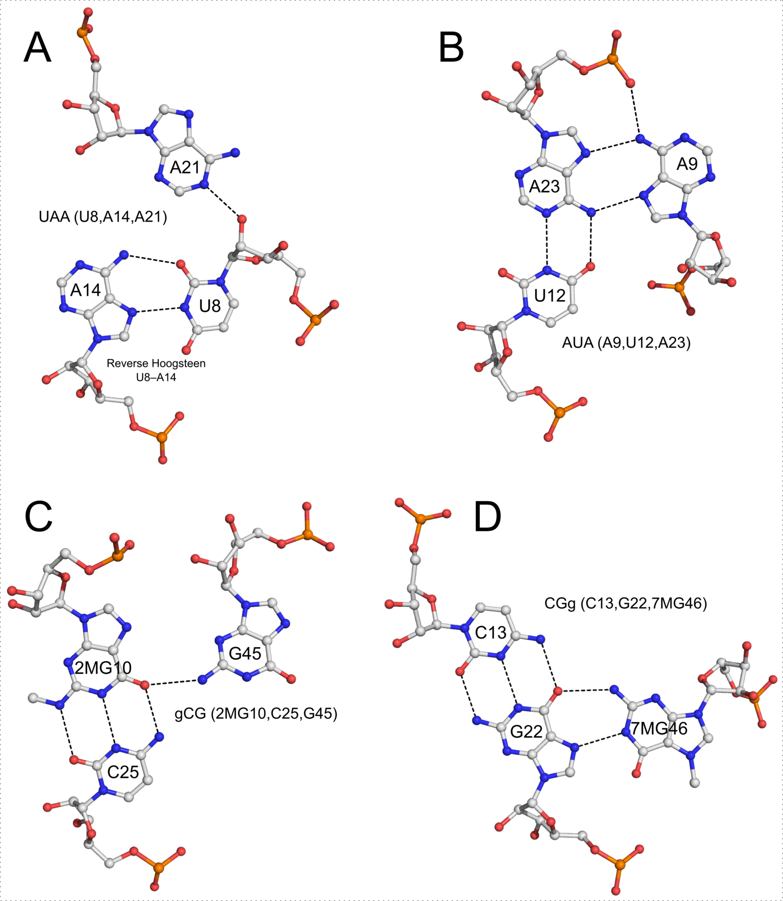
In addition to base pairs, DSSR also automatically detects higher-order base associations. They are generally termed multiplets, consisting of three or more co-planar bases arranged together via H-bonding interactions. The simplest multiplets are base triplets. For example, the yeast phenylalanine tRNA (PDB entry 1ehz) contains four base triplets, as shown below:

The well-known (types I and II) A-minor motifs are also multiplets of three bases. Similarly, the G-tetrad where four guanine bases associate via Hoogsteen H-bonding to form a square planar structure is also a special multiplet. The G-tetrad is the building block of the G-quadruplexes. As of v1.7.0-2017oct19, DSSR can automatically identify and characterize G-quadruplexes (see the DSSR User Manual).

The DSSR algorithm for detecting multiplets is generally applicable. It can identify as many co-planar bases as available in a given structure. Shown below is an octad, consisting of a G-tetrad in the middle and four Us on the peripheries. The octad is derived from PDB entry 1j8g using atomic coordinates from biological assembly 1 and 3.

The DSSR-Jmol paper, titled "DSSR-enhanced visualization of nucleic acid structures in Jmol", has been officially published in the 2017 web-server issue of Nucleic Acids Research (NAR). Notably, the work has been featured in the cover image, as shown below:

Caption: 3D interactive visualization of selected RNA structural features enabled by the DSSR-Jmol integration (http://jmol.x3dna.org). Clockwise from upper left: Structure of the xpt-pbuX guanine riboswitch in complex with hypoxanthine (PDB id: 4fe5) in ‘base blocks’ representation. The three-way junction loop encompassing the metabolite (in space-filling representation) is color-coded by base identity: A, red; C, yellow; G, green; U, cyan. The loop-loop interaction (a kissing-loop motif) at the top is highlighted in red (upper left corner). Structure of the Thermus thermophilus 30S ribosomal subunit in complex with antibiotics (PDB id: 1fjg) in step diagram. The 16S ribosomal RNA is color-coded in spectrum with the 5′-end in blue and the 3′-end in red (upper middle). Structure of the classic L-shaped yeast phenylalanine tRNA (PDB id: 1ehz) in step diagram, with the three hairpin loops highlighted in red and the [2,1,5,0] four-way junction loop in blue (upper right corner). Structure of the Pistol self-cleaving ribozyme (PDB id: 5ktj), showcasing (in red) the horizontal helix in space-filling representation. The helix is composed of six short stems stabilized via coaxial stacking interactions (bottom).

The DSSR-Jmol integration bridges the DSSR command-line analyzing tool and the Jmol molecular viewer seamlessly together via the standard JSON interface. Now users can select DSSR-derived RNA structural features (such as base pairs, double helices, various loops, etc.) and visualize them in novel representations in Jmol interactively. Moreover, fine-grained characteristics of these features can be queried via the Jmol SQL for DSSR. The DSSR-Jmol integration fills a gap in RNA structural bioinformatics, and brings RNA visualization to an entirely new level. The web interface (http://jmol.x3dna.org) is fully functional and easy to use, serving a huge user base of researchers, educators, and students alike.

Featured as the cover image of the 2017 NAR web-server issue, DSSR's publicity would surely increase through the DSSR-Jmol integration. Additionally, I've written a new post (on the 3DNA Forum) that provides the scripts and datafiles used to create the cover image.

I am pleased to announce the (advance online, May 3, 2017) publication of a new paper titled "DSSR-enhanced visualization of nucleic acid structures in Jmol" in Nucleic Acids Research (NAR). Co-authored by Robert Hanson (Jmol) and me (DSSR), the article will appear in the July 2017 web-server issue of NAR. Here are the key links related to the paper:

• DSSR-Jmol website
• PDF version (DSSR-Jmol paper)
• Online HTML (DSSR-Jmol paper)
• DSSR-Jmol manual
• Materials to reproduce reported results

The DSSR-Jmol integration project was initiated in October 2013 when I approached Bob at a meeting organized by RCSB PDB at Rutgers. Thereafter, we met only once in July 2014 in Paris. Over the years, we have mostly communicated via email, occasionally facilitated by Skype. Our work bridges the DSSR command-line analyzing tool and the Jmol molecular viewer together via a simple JSON interface and a powerful query language. Users can now select DSSR-derived RNA structural features (such as base pairs, double helices, and various loops) as easily as they can select protein alpha-helices and beta-strands. Moreover, fine-grained characteristics of these features can be queried via Jmol SQL for DSSR (see examples below). Notably, the novel representation styles (step diagram and base blocks) and coloring schemes bring RNA visualization to an entirely new level (see Figure 3 of the paper).

load =1ehz/dssr   # load yeast phenylalanine tRNA to Jmol with DSSR annotation
SELECT hairpins   # select the three hairpin loops
SELECT junctions  # select the four-way junction loop
select within(dssr, "nts WHERE is_modified")  # select modified nucleotides (14 total)
SELECT within(dssr, "pairs WHERE name != 'WC'")  # select non-Watson-Crick pairs
SELECT within(dssr, "pairs WHERE name = 'WC' OR name = 'Wobble'")  # select canonical pairs
Select within(dssr, "pairs WHERE name != 'WC' AND name != 'Wobble'")  # select non-canonical pairs
SELECT within(dssr, "pairs WHERE LW = 'tSW'")  # select pairs of type tSW per Leontis-Westhof

The DSSR-Jmol integration fills a gap in RNA structural bioinformatics, serving a huge user base of researchers, educators, and students alike. Its functionality is freely accessible either via the Jmol application, or the JSmol-based website (http://jmol.x3dna.org). By adhering to web standards, the website is fully functional in all modern browsers on various computer/operating systems (including handheld devices, such as tablets and smart phones). The web interface is simple and intuitive, and new users can get started easily. It also allows power users to take full advantage of Jmol scripting via a command-line console.

This work also provides an example for integrating DSSR-derived features into other molecular graphics programs or bioinformatics pipelines involving nucleic acid structures. By design, DSSR is a stand-alone, command-line program written in ANSI C. The binary executables are only ~1MB in size, and self-contained. With zero dependencies, no setup or configuration, it is trivial to get DSSR up and running. DSSR uncovers a wide range of RNA/DNA structural features in a consistent, easily accessible framework. It possesses a much richer set of functionalities for nucleic acid structural analysis (see the DSSR User Manual) than any other existing tools I am aware of. Moreover, the program is efficient and robust, making it an ideal component to be integrated into other pipelines, especially via the standard and structured JSON interface.

Collaborating with Bob has been a truly exciting experience. The NAR-web publication represents a gratifying intermediate result along an on-going journey. Hopefully, others (may be some of you) can join us in pushing forward the field of RNA structural bioinformatics.