[Job] Staff Associate II (Computational Structural Biology) at Columbia University
The X3DNA-DSSR resource is at the forefront of structural bioinformatics, developing advanced tools for analyzing and modeling nucleic acid structures. We are seeking a highly motivated Staff Associate II to join our team and contribute to our next-generation analysis and visualization engine.
To see our resource in action, please visit wDSSR, our new web interface for dissecting and modeling 3D nucleic acid structures: https://web.x3dna-dssr.org/.
We are looking for a candidate with a strong scientific background in structural biology or bioinformatics and a desire to contribute to peer-reviewed publications through community-driven data analysis. We value individuals who are eager to learn, adapt to new technical challenges, and support the global research community.
For the full job description and to submit your application, please visit the official Columbia University posting:
https://apply.interfolio.com/183705
Announcing wDSSR: The Next-Generation Web Interface to X3DNA-DSSR
Dear 3DNA/DSSR Community,
We are thrilled to announce the official launch of wDSSR (https://web.x3dna-dssr.org/), the powerful new web interface to the X3DNA-DSSR analytical engine.
Developed by Drs. Shuxiang Li and Xiang-Jun Lu and supported by NIH grant R24GM153869, wDSSR represents a major leap forward from our highly popular 2019 Web 3DNA 2.0 framework. While Web 3DNA 2.0 has faithfully served the community for the analysis, visualization, and modeling of 3D nucleic acid structures, wDSSR was built from the ground up to take full advantage of modern web technologies and the latest DSSR backend capabilities.
A Modern, Streamlined Scientific Workflow
We have completely overhauled the user interface to provide a clean, intuitive, and task-driven experience. The core modeling and analysis tools are now seamlessly organized into a logical, single-word scientific workflow: Analyze, Rebuild, Model, Circularize, Mutate, Assemble, and Visualize.
Spotlight Feature: The "Assemble" Module
One of the most exciting upgrades is the newly renamed Assemble tab (formerly "Composite"). This advanced composite model builder allows you to effortlessly construct complex, higher-order models by linking any combination of nucleic acid duplexes or protein-DNA/RNA complexes. You can quickly connect up to six distinct target structures, ranging from simple linked A-DNA and B-DNA duplexes to large, protein-decorated structural assemblies.
Immediate Global Adoption
Although wDSSR has just launched, we are incredibly humbled to share that it is already seeing rapid worldwide adoption! According to recent network infrastructure data, the new interface is actively being used by researchers across North America, South America, Europe, and Asia. Within just a few days, we have recorded active sessions from prestigious institutions around the globe, including:
- The Weizmann Institute of Science in Israel
- Katholieke Universiteit Leuven in Belgium
- Queen's University in Canada
- Universidad Nacional Autonoma de Mexico (UNAM) in Mexico
- Emory University and the Wadsworth Centers Laboratories and Research in the United States
- Jawaharlal Nehru University and the China Education and Research Network in Asia
How to Cite
While a dedicated paper for wDSSR is currently in preparation, researchers should cite the server using its URL (https://web.x3dna-dssr.org/) alongside the 2019 Web 3DNA 2.0 paper and the foundational 2015 DSSR paper. Full details and funding acknowledgements can be found on our newly consolidated About page.
We invite you all to try out the new wDSSR platform! As always, your feedback is invaluable to us, and we encourage you to share your thoughts, questions, and structural models via the newly updated Questions & Feedback link in the wDSSR footer.
Happy modeling!
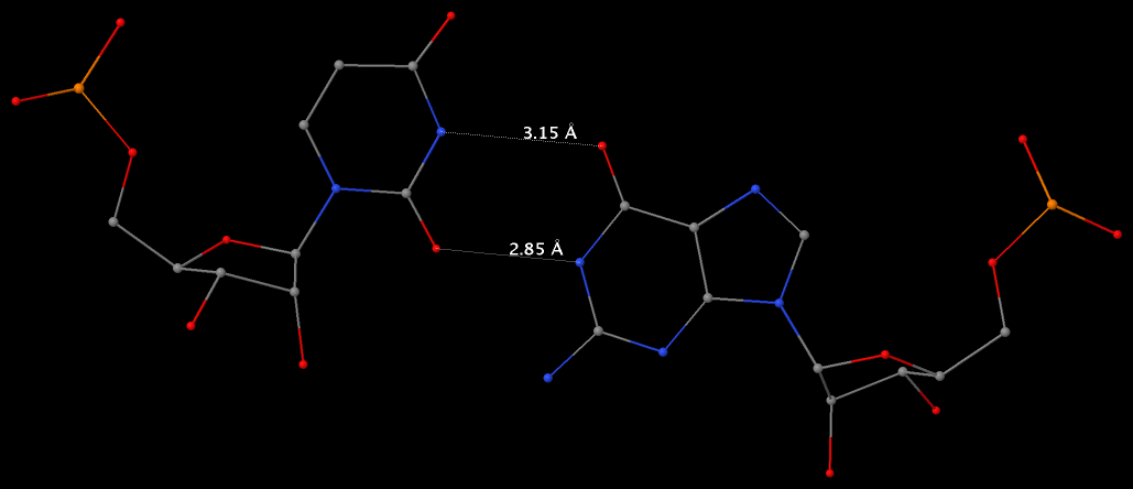
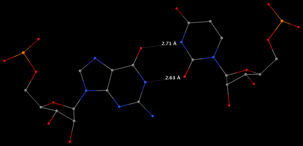
Among the findings of our 2010 Nucleic Acids Research (NAR) article titled The RNA backbone plays a crucial role in mediating the intrinsic stability of the GpU dinucleotide platform and the GpUpA/GpA miniduplex, the key is identifying the O2′(G)…O2P(U) H-bond (see figure below). As noted in a previous post What’s special about the GpU dinucleotide platform?, it was an accidental observation while I was preparing a figure for our 2008 3DNA Nature Protocols paper. Trained as a chemist, after scrutinizing the many occurrances of the GpU platforms in the large ribosomal subunit of Haloarcula marismortui (PDB entry 1jj2), I had no doubt that it is an H-bond. Yet, behind the scene, things were never that straightforward: if it is indeed an H-hbond as we’ve claimed, how could it have been missed altogether by the RNA structural biology community?
...O2P(U) H-bond in the sugar–phosphate backbone.")
Anticipating the potential questions that could be raised by the reviewers, we were extremely careful in characterizing the O2′(G)…O2P(U) H-bond:
- It is formed between the hydroxyl group (donor) of G and a non-bridging phosphate oxygen atom (O2P, acceptor) of U.
- The distance between O2′(G) and O2P(U), 2.68 ± 0.14 Å, is perfect for an H-bond.
- I queried the Cambridge Structure Database for hydroxyl-phosphate H-bonds with similar relative geometry and chemical identity. We found a case in the phospholipid lysophosphatidyl-ethanolamine, where this type of H-bond is highlighted in the abstract: The free glycerol hydroxyl group forms an intramolecular hydrogen bond with a phosphate oxygen and thus affects the conformation and orientation of the head group.
- I also performed a survey of potential O2′(i)…O2P(i+1) H-bonds within dinucleotides regardless of platform configuration, and detected 1186 such pairwise interactions within a distance cutoff of 3.3 Å in RNA crystal structures of 2.5 Å or better resolution.
Careful as we were, we still failed to convince reviewer #3 of our manuscript, which was originally submitted to the RNA journal and finally rejected following the second round of review. Here is an excerpt related to the O2′(G)…O2P(U) H-bond from reviewer #3’s comment:
The first main concern is that the “new” H-bond interaction that the authors propose as an explanation for the greater occurrence of GU platforms versus di-nucleotide combinations does not make much sense on a fundamental chemical and stereo-chemical point of view. Unless the whole community of chemists and biochemists agree to redefine what an H-bond is, the fact that the 2’OH (i) atom is at 2.68 Å from the O2P atom cannot be the only criteria for an H-bond. In fact, if the authors are the first to mention this H-bond, it is because none of the scientists working in RNA structural biology would have considered this to be an H-bond interaction at the first place! H-bonds are known to be very directional. The O2’-H bond should be aligned with one of the electron doublets of O2P to be able to form a proper H-bond. Acceptable variation could be 20° to 30° degree with respect of a straight H-bond interaction, not 90°! The unique paper that the authors cite for justifying their claim cannot be used as a reference. If the authors want to justify that the close proximity of the 2’OH(i) and O2P is the important factor that contributes to preference of GU platforms versus other platforms, they should undergo quantum mechanics calculations to demonstrate it.
This review is so critical that I saw no point in arguing with it — I certainly have neither the power to “redefine what an H-bond is” nor the expertise to perform quantum mechanics (QM) calculations to validate the O2′(G)…O2P(U) H-bond or otherwise. What is compelling to me about the GpU story from the very beginning is that once this sugar-phosphate H-bond is acknowledged, every other parts of our NAR paper follow naturally and logically. Leaving the chicken or the egg issue alone, our work provides a novel perspective about GpU platform’s predominance, the formation of the bulged-G or loop-E motif, the evolutionary co-occurrence of GpUpA and GpA in the GpUpA/GpA miniduplex, and the extreme conservation of GpU observed at most 5′-splice sites. Put another way, we connect the dots to form a coherent picture that is easily understandable to biologists and chemists.
Luckily, after being re-submitted to NAR, the paper was quickly accepted for publication and even selected as a featured article! As another nice surprise, shortly after it was available online as an Advance Access paper, I received an email from Jiri Sponer. Thereafter, we collaborated on a follow-up paper titled Understanding the Sequence Preference of Recurrent RNA Building Blocks Using Quantum Chemistry: The Intrastrand RNA Dinucleotide Platform. While not unexpected, the results of the state-of-the-art QM calculations were nevertheless reassuring:
The mixed-pucker sugar–phosphate backbone conformation found in most GpU platforms, in which the 5′-ribose sugar (G) is in the C2′-endo form and the 3′-sugar (U) in the C3′-endo form, is intrinsically more stable than the standard A-RNA backbone arrangement, partially as a result of a favorable O2′···O2P intraplatform interaction. Our results thus validate the hypothesis of Lu et al. (Lu, X.-J.; et al. Nucleic Acids Res. 2010, 38, 4868–4876) that the superior stability of GpU platforms is partially mediated by the strong O2′···O2P hydrogen bond. …… In contrast, we show that the dinucleotide platform is not properly described in the course of atomistic explicit-solvent simulations. Our work also gives methodological insights into QM calculations of experimental RNA backbone geometries. Such calculations are inherently complicated by rather large data and refinement uncertainties in the available RNA experimental structures, which often preclude reliable energy computations.
So, the O2′(G)…O2P(U) H-bond is more than likely to be real; at least some other scientists working in RNA structural biology do share our view.
See also: What’s special about the GpU dinucleotide platform?

While the Watson-Crick (WC) base pairs (bps) are best-known and most abundant in nucleic acid structures (including RNA), the so-called reverse WC bp variants have received little attention. In the well-established Saenger scheme (see figure below), there are 28 possible bps for A, G, U(T), and C in their cononical (keto- and amino-) tautomeric forms and involving at least two H-bonds. The reverse A·T/U and G·C WC pairs are asymmetric, and are numbered XXI and XXII respectively (middle of right-hand side in the figure below).

In 3DNA, the WC bps are of type M–N and listed as A–T and G–C, consistent with the conventional notation. The reverse WC bps, on the other hand, are of type M+N and listed as A+T and G+C; the ‘+’ signifies the parallel z-axes of the two base reference frames, therefore their dot product is positive (see figure 2 in post Hoogsteen and reverse Hoogsteen base pairs).
As of this writing, a Google search of the phrase “reverse Watson Crick base pair” does not come up with anything informative — the top hit is the Jena Library page titled Nucleic Acid Nomenclature and Structure showing the same set of 28 possible bps only with explicit base chemical structures, as compiled by Tinoco Jr. et al. (1993).
However, once I look into this special type of bps, a quick search in PDB entry 1jj2, the Haloarcula marismortui large ribosomal subunit solved at 2.4 Å resolution, revealed nine reverse WC bps as shown below:
 __U.U..0.205._   __A.A..0.437._   [U+A]
 __C.C..0.1186._  __G.G..0.1190._  [C+G]
 __C.C..0.1377._  __G.G..0.1683._  [C+G]
 __C.C..0.1856._  __G.G..0.1873._  [C+G]
 __A.A..0.2054._  __U.U..0.2648._  [A+U]
 __U.U..0.2109._  __A.A..0.2467._  [U+A]
 __A.A..0.2301._  __U.U..0.2306._  [A+U]
 __A.A..0.2321._  __U.U..0.2378._  [A+U]
 __C.C..0.2510._  __G.G..0.2564._  [C+G]
The following figure shows a representative reverse WC A+U bp (0.A437 with 0.U205, top), and a representative reverse WC G+C bp (0.G1683 with 0.C1377, bottom). For easy comparison, the two reverse WC bps are orientated in the reference frames of A and G, respectively.
In future releases of 3DNA, presumably starting from v2.2, we plan to provide a new component to classify bps according to the Saenger scheme, the Leontis/Westhof notation, and the geometric parameter-based strategy. Overall, the three bp classification methods are complementary in functionality, but with increased sophistication and applicability.
The A·U (or A·T) Hoogsteen pair is a well-known type of base pair (bp), named after the scientist who discovered it. As shown in the Figure below (left), in the Hoogsteen bp scheme, adenine uses its N7 (acceptor) and N6 (donor) atoms at the major groove edge to form two H-bonds with the N3 (donor) and O4 (acceptor) atoms from uracil, respectively. Interestingly, if the uracil base ring is flipped around the N7(A)…N3(U) H-bond by 180 degrees, N6(A) now forms an H-bond with O2(U), i.e., N6(A)…O2(U): this pairing scheme is called the reverse Hoogsteen bp (right).

I first knew about the Hoogsteen bp from Saenger’s book titled “Principles of Nucleic Acid Structure”. My knowledge of the Hoogsteen bp deepened as I tried to categorize different types of bps, especially in RNA-containing structures, in a consistent and rigorous computational framework. Thus, in the 3DNA NAR03 publication, we discussed specifically the bp (M+N type) and compared it with the A·U Watson-Crick bp (M–N type), as shown in the Figure below:

Antiparallel and parallel combinations of adenine (A) and uracil (U) base pair ‘faces’: (a) the antiparallel Watson–Crick A–U pair with opposing faces (shaded versus unshaded) and a 1.5 Å Stretch introduced to separate the two base reference frames; (b) the parallel Hoogsteen A+U pair with base pair faces of the same sense. Black dots on bases denote the C1′ atoms on the attached sugars.
However, only recently did I read the two original publications by Hoogsteen:
- The two-page long preliminary report, titled The structure of crystals containing a hydrogen-bonded complex of 1-methylthymine and 9-methyladenine [Acta Cryst. (1959). 12, pp.822-3]. It contains only a single reference, i.e. the 1953 Watson-Crick DNA structure Nature paper. Reading carefully through the two pages, I know why Hoogsteen used the methylated derivatives of thymine and adenine, and how the failed initial interpretation of the experimental “vector-density map” based on the Watson-Crick A-T bp led to the discovery of the new base-pairing scheme:
The fact that the first trial structure could not be refined led to a more critical scrutiny of the generalized projection and a greater emphasis on the significance of certain spurious peaks and on relatively large variations in the heights of peaks that were assumed to represent atoms. The correct structure was finally discovered by changing the positions of a few atoms in the 9-methyladenine portion of the asymmetric unit.
I enjoyed reading these two papers a lot. More generally, I like such focused articles where authors get directly to a point and addressed it thoroughly and clearly.
As a side note, the term Hoogsteen “edge” appears frequently in nowaday’s publications of RNA structures: in the Leontis-Westhof bp classification scheme, this term simply means the major groove edge in what would be a Watson-Crick bp geometry.
3DNA, following SCHNArP, uses the alchemy file format for the schematic base-pair rectangular block representation. Alchemy is a simple molecular file format, suitable for chemical compounds by specifying atom positions and bond linkages explicitly. By checking a sample alchemy file (here for drug aspirin), scientists with chemistry knowledge should have little problem in figuring out what each field means. As it happens, the 3DNA alchemy representation of the base-pair rectangular block is much simpler than that of a typical chemical compound (e.g., aspirin). No different partial atomic charges or atom types, no distinction between single-, double- or aromatic bond types, the base-pair block can be specified with uniform pseudo-atoms (nodes) and pseudo-bonds (edges). Apart from being simple, alchemy was one of the common file formats supported by RasMol — that’s the pragmatic reason why I adopted the format in SCHNArP and 3DNA.
Over the years, 3DNA has been continuously using the alchemy format for base and base-pair rectangular blocks. It forms the basis of the Calladine-Drew style schematic representation images in PostScript (.eps), Xfig (.fig) and Raster3d (.r3d) formats. However, outside 3DNA, the alchemy format is not widely supported by popular molecular graphics programs, including RasMol, Jmol and PyMOL:
- RasMol v2.6.4, from Roger Sayle (the original author of RasMol), is mostly fine, except that the
-noconnect option should be specified. As noted in the 3DNA Nature Protocols (2008) paper, The option ‘-noconnect’ makes sure that RasMol uses only the linkage information specified in the Alchemy file (by setting the CalcBondsFlag to false). … The … Alchemy files [can] contain explicitly specified coordinate axes, which would interfere with the default bond-calculation algorithm in RasMol.
- RasMol v2.7.x has a bug in displaying alchemy files.
- Jmol begins to support the alchemy format as of 11.7.18 (December 2008), following my request [see initial discussion and follow-up].
- PyMOL does not recognize the alchemy format.
To make the schematic base-pair rectangular block representation more broadly accessible, I have recently added the -mol option to alc2img in 3DNA v2.1 to readily convert an alchemy file to the well-documented and widely supported MDL molfile format. The usage is very simple — take the standard base-pair rectangular block file (Block_BP.alc) as an example, the conversion can be performed as below:
alc2img -mol Block_BP.alc Block_BP.mol
alc2img -molv3000 Block_BP.alc Block_BP_v3000.mol
Note the followings:
- By default, the
-mol option converts alchemy to V2000 molfile format. However, if the number of atoms/bonds is greater then 999, the extended V3000 molfile format is used.
- The V3000 molfile format can be explicitly specified with
-molv3000 (or -mol3), as shown above.
- Only V2000 molfile is consistently supported by RasMol, Jmol and PyMOL. On the other hand, while Jmol recognizes V3000 molfile, RasMol and PyMOL do not.
- For reference, the three files — Block_BP.alc, Block_BP.mol, and Block_BP_v3000.mol — are enclosed below.
Content of ‘Block_BP.alc’
   12 ATOMS,    12 BONDS
    1 N      -2.2500   5.0000   0.2500
    2 N      -2.2500  -5.0000   0.2500
    3 N      -2.2500  -5.0000  -0.2500
    4 N      -2.2500   5.0000  -0.2500
    5 C       2.2500   5.0000   0.2500
    6 C       2.2500  -5.0000   0.2500
    7 C       2.2500  -5.0000  -0.2500
    8 C       2.2500   5.0000  -0.2500
    9 C      -2.2500   5.0000   0.2500
   10 C      -2.2500  -5.0000   0.2500
   11 C      -2.2500  -5.0000  -0.2500
   12 C      -2.2500   5.0000  -0.2500
    1     1     2
    2     2     3
    3     3     4
    4     4     1
    5     5     6
    6     6     7
    7     7     8
    8     5     8
    9     9     5
   10    10     6
   11    11     7
   12    12     8
Content of ‘Block_BP.mol’ (V2000)
Block_BP.alc
XL 3DNAv2
Converted from Alchemy format: Thu May  3 23:35:20 2012
 12 12  0     0  0              1 V2000
   -2.2500    5.0000    0.2500 N   0  0  0  0  0  0  0  0  0  0  0  0
   -2.2500   -5.0000    0.2500 N   0  0  0  0  0  0  0  0  0  0  0  0
   -2.2500   -5.0000   -0.2500 N   0  0  0  0  0  0  0  0  0  0  0  0
   -2.2500    5.0000   -0.2500 N   0  0  0  0  0  0  0  0  0  0  0  0
    2.2500    5.0000    0.2500 C   0  0  0  0  0  0  0  0  0  0  0  0
    2.2500   -5.0000    0.2500 C   0  0  0  0  0  0  0  0  0  0  0  0
    2.2500   -5.0000   -0.2500 C   0  0  0  0  0  0  0  0  0  0  0  0
    2.2500    5.0000   -0.2500 C   0  0  0  0  0  0  0  0  0  0  0  0
   -2.2500    5.0000    0.2500 C   0  0  0  0  0  0  0  0  0  0  0  0
   -2.2500   -5.0000    0.2500 C   0  0  0  0  0  0  0  0  0  0  0  0
   -2.2500   -5.0000   -0.2500 C   0  0  0  0  0  0  0  0  0  0  0  0
   -2.2500    5.0000   -0.2500 C   0  0  0  0  0  0  0  0  0  0  0  0
  1  2  1  0  0  0
  2  3  1  0  0  0
  3  4  1  0  0  0
  4  1  1  0  0  0
  5  6  1  0  0  0
  6  7  1  0  0  0
  7  8  1  0  0  0
  5  8  1  0  0  0
  9  5  1  0  0  0
 10  6  1  0  0  0
 11  7  1  0  0  0
 12  8  1  0  0  0
M END
Content of ‘Block_BP_v3000.mol’ (V3000)
Block_BP.alc
XL 3DNAv2
Converted from Alchemy format: Thu May  3 23:22:04 2012
  0  0  0     0  0            999 V3000
M  V30 BEGIN CTAB
M  V30 COUNTS    12    12 0 0 0
M  V30 BEGIN ATOM
M  V30     1 N     -2.2500     5.0000     0.2500 0
M  V30     2 N     -2.2500    -5.0000     0.2500 0
M  V30     3 N     -2.2500    -5.0000    -0.2500 0
M  V30     4 N     -2.2500     5.0000    -0.2500 0
M  V30     5 C      2.2500     5.0000     0.2500 0
M  V30     6 C      2.2500    -5.0000     0.2500 0
M  V30     7 C      2.2500    -5.0000    -0.2500 0
M  V30     8 C      2.2500     5.0000    -0.2500 0
M  V30     9 C     -2.2500     5.0000     0.2500 0
M  V30    10 C     -2.2500    -5.0000     0.2500 0
M  V30    11 C     -2.2500    -5.0000    -0.2500 0
M  V30    12 C     -2.2500     5.0000    -0.2500 0
M  V30 END ATOM
M  V30 BEGIN BOND
M  V30     1 1    1    2
M  V30     2 1    2    3
M  V30     3 1    3    4
M  V30     4 1    4    1
M  V30     5 1    5    6
M  V30     6 1    6    7
M  V30     7 1    7    8
M  V30     8 1    5    8
M  V30     9 1    9    5
M  V30    10 1   10    6
M  V30    11 1   11    7
M  V30    12 1   12    8
M  V30 END BOND
M  V30 END CTAB
M END
In the standard base reference frame report, a whole section is devoted to the discussion of intrinsic correlations between base-pair and dimer step parameters (see figure below). Among the four sets of associations, the effect of Δbuckle (difference in consecutive base-pair buckles) on rise is most noticeable and easiest to understand. The Δshear vs. twist relationship is similarly significant, due to its close connection to the wobble G–T/G–U pair; yet the concept is less comprehensible, especially to occasional 3DNA users. This post aims to address the issue of how Δshear effects twist.

Under the standard base reference frame used in 3DNA, the wobble base-pair has a ~2.0 Å shear: the displacement is positive for U–G, and negative for G–U [see figure below, examples selected from 5S rRNA (chain 9) U82–G100 and G83–U99 of the Haloarcula marismortui large ribosomal subunit, PDB id: 1jj2].
As noted in the section “treatment of non-Watson–Crick base pairing motifs” of the 3DNA Nucleic Acids Research paper (2003), “Large Shear of the G–U wobble base pair influences the calculated but not the ‘observed’ Twist. The 3DNA numerical values of Twist [of the C7G8·U12G13 and G8C9·G11U12 dimer steps of the Escherichia coli tRNAAsp x-ray crystal structure (PDB id: 485d)], 20° (top) and 43° (bottom), differ from the visualization of nearly equivalent Twist suggested by the angle between successive C1′···C1′ vectors (finely dotted lines).”

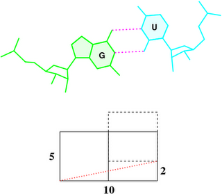
To make it clear why that’s the case, the figure below shows a G–U wobble pair in atomic representation (top), and a schematic base pair rectangular block of dimension 10×5 (Å, bottom). A shear of –2 Å moves U upwards, as outlined by the dashed rectangle, and causes a ‘misalignment’ of 11.3° between the C1′···C1′ vector (red dotted line) and the base-centered mean y-axis (horizontal line):
atan2(2, 10) * 180 / pi = 11.3°
To a first order approximation, that is the difference in twist angle. So whenever a wobble pair is next to a normal Watson-Crick pair, there would be a ~11° “observed” discrepancy with 3DNA calculated twist angle. Moreover, when a G–U wobble is next to a U–G wobble pair or vice versa, the difference would be doubled to ~22°.
The blocview script in 3DNA has been created as a handy tool to effectively reveal key features of small to medium-sized nucleic acid structures. Specifically, the bloc part of the name means ‘block’, i.e., the rectangular block in Calladine-Drew style schematic representation to distinguish bases by size (larger purine vs. smaller pyrimidine), identity (red for A, yellow for C, green for G, and blue for T), and groove (minor edge in black). The view part stands for the most extended view, as defined by the principal axes of inertia. Implementation-wise, blocview calls several 3DNA utility programs and MolScript (for protein ribbons and nucleic acid backbone rods) to prepare the scenes, and then uses Raster3D (specifically, render) or PyMol to generate a PNG image.
The blocview script was originally written in Perl. As of 3DNA v2.1, I decided to switch the scripting language to Ruby for its consistent object-oriented style, succinct and flexible syntax. Previously available Perl scripts are now moved out of the default 3DNA executable directory $X3DNA/bin/ into $X3DNA/perl_scripts/. The blocview script has been re-written in Ruby and set as the default (at $X3DNA/bin/blocview); the original Perl version is renamed blocview.pl (at $X3DNA/perl_scripts/blocview.pl) to avoid confusion. The command line help message, available via blocview -h, is as below:
------------------------------------------------------------------------
Generate a schematic image which combines base block representation
with protein ribbon. The image has informative color coding for the
nucleic acid part and is set in the "best view" by default. Raster3D
(or PyMOL) and ImageMagick must be installed.

Usage:
        blocview [options] PDBFile
Examples:
        blocview -i 355d.png 355d.pdb
             # generate image '355d.png'; display 355d.png
Options:
------------------------------------------------------------------------
     --imgfile, -i <s>:   name of image file (default: blocview.png)
     --r3dfile, -r <s>:   name of .r3d file (default: blocview.r3d)
   --dpi-pymol, -d <i>:   create PyMOL ray-traced image at specific DPI
       --scale, -s <f>:   set scale factor (for 'render' of Raster3D)
        --xrot, -x <f>:   rotation angle about x-axis
        --yrot, -y <f>:   rotation angle about y-axis
        --zrot, -z <f>:   rotation angle about z-axis
        --original, -o:   use original coordinates
  --ball-and-stick, -b:   get a ball-and-stick image
     --p-base-ring, -c:   use only P and base ring atoms
           --no-ds, -n:   do not show double-helix ribbon
         --protein, -p:   set best view based on protein atoms
             --all, -a:   set best view based on all atoms
         --version, -v:   Print version and exit
            --help, -h:   Show this message
Using the x-ray crystal structure of d(GGCCAATTGG) complexed with netropsin (1z8v) in the minor groove as an example, the command to run is as follows:
blocview -i 1z8v.png 1z8v.pdb
# The following two forms are also fine
#     blocview --imgfile 1z8v.png 1z8v.pdb
#     blocview --imgfile=1z8v.png 1z8v.pdb
# The Perl version can be run like this:
#     $X3DNA/perl_scripts/blocview.pl -i=1z8v.png 1z8v.pdb
The image, named 1z8v.png, is shown below. Note that it is generated automatically from the PDB-formatted data file 1z8v.pdb. In this representation, one can see clearly that there are two unpaired Gs (green block) at each 5′-end of the two DNA chains (red and yellow rods), and a drug molecule (ball-and-stick) binds in the minor groove (black edge of the rectangular blocks). Moreover, the deformation in propeller and buckle is obvious in this schematic presentation.

Over the years, blocview-generated images have been used in NDB for virtually all nucleic acid structures (see for example, the NDB atlas gallery for x-ray drug-DNA complexes). It’s worth noting that such simple images have also be adopted by the RCSB PDB, prominently at the summary page, for nucleic acid containing structures (see PDB entry 1z8v). Given the effectiveness of blocview-generated schematic representation and its adoption by the NDB and PDB, I’m hopeful that blocview will be more widely used by the general DNA/RNA structure community. As always, I value user’s feedback in continuously refining the script.
One of 3DNA’s unique features is the simplified rectangular block representation of bases and base-pairs, as shown in the figure below. This type of schematic depiction was first made popular by Calladine and Drew (see their book titled Understanding DNA — The Molecule & How It Works), thus I usually call it the Calladine-Drew style representation.

By default, a base-pair [BP, (a)] has dimensions of 10×4.5×0.5 (Å); a purine [R, (b) left] 4.5×4.5×0.5 (Å); a pyrimidine [Y, (b) right] 3×4.5×0.5 (Å); and a mean base [M, (c)], which is exactly half of the base-pair, 5×4.5×0.5 (Å).
The blocks are stored into separate files: Block_BP.alc, Block_R.alc, and Block_Y.alc for BP, R and Y respectively. To use M for R and Y (i.e., set R and Y to be of equal size), simple copy file Block_M.alc to overwrite Block_R.alc and Block_Y.alc in the current working directory for local effect, or the 3DNA installation directory ($X3DNA/config/) for global impact. These blocks are used in the rebuilding and visualization components of 3DNA.
Following SCHNArP, 3DNA uses alchemy, a simple chemical file format, to specify explicitly the nodes (atoms) and edges (bonds) of a rectangular block. Three file formats (alchemy, MDL molfile, and Tripos mol2), supported by RasMol v2.6 (the most popular molecular graphics visualization program in the 1990s), serve the purpose of specifying the rectangular block. I cannot recall exactly why I picked up -alchemy instead of -mdl and -mol2, perhaps because of its simplicity: I played around with sample alchemy files and came up with the alchemy rectangular block files used by SCHNArP, without much difficulty.
As an example, Block_BP.alc has the following content:
   12 ATOMS,    12 BONDS
    1 N      -2.2500   5.0000   0.2500
    2 N      -2.2500  -5.0000   0.2500
    3 N      -2.2500  -5.0000  -0.2500
    4 N      -2.2500   5.0000  -0.2500
    5 C       2.2500   5.0000   0.2500
    6 C       2.2500  -5.0000   0.2500
    7 C       2.2500  -5.0000  -0.2500
    8 C       2.2500   5.0000  -0.2500
    9 C      -2.2500   5.0000   0.2500
   10 C      -2.2500  -5.0000   0.2500
   11 C      -2.2500  -5.0000  -0.2500
   12 C      -2.2500   5.0000  -0.2500
    1     1     2
    2     2     3
    3     3     4
    4     4     1
    5     5     6
    6     6     7
    7     7     8
    8     5     8
    9     9     5
   10    10     6
   11    11     7
   12    12     8
Observant viewers may notice that nodes 1-4 are specified as nitrogens (N) which have exactly the same coordinates as 9-12 (carbons, C). This is a little trick to make RasMol display the minor groove edge in a different color (blue for N) than the other five sides of the rectangular (gray for C), as shown in the following figure:

Note that the rectangular is preset in the standard base reference frame. Thus the nodes have y-coordinates of +5 Å and -5 Å along the long edge of the base pair, and x-coordinates of +2.25 Å and -2.25 Å along the short edge.
As an extra bonus of storing the rectangular blocks in external alchemy text files, the dimensions of the blocks can be readily changed. For example, the thickness of a block (z-coordinates) can be easily increased from 0.5 to 1.0 Å to make it thicker. Moreover, the blocks do not need to be rectangular either — they can appear to be triangular blocks.
It’s worth noting that while extensively used in 3DNA for schematic representations, the alchemy format has largely become a legacy in cheminformatics/bioinformatics nowadays. Searching the internet, I cannot find the specification of the format. Moreover, the support of alchemy is quite limited and buggy in molecular graphics visualization programs most widely used today: PyMOL does not understand this format at all; RasMol v2.7 has a bug in interpreting it; only Jmol can properly read 3DNA base-pair rectangular block files in alchemy [see initial discussion and follow-up]. To resolve the issues associated with alchemy format, and thus to make 3DNA base-pair block schematics more widely available, I have recently added a converter in v2.1 to readily transform alchemy to MDL molfile, a format consistently supported by PyMOL, Jmol and RasMol. I’ll talk about this feature in another post.
The conformation of the five-membered sugar ring in DNA/RNA structures can be characterized by the five consecutive endocyclic torsion angles (see Figure below), i.e.,
ν0: C4′-O4′-C1′-C2′
ν1: O4′-C1′-C2′-C3′
ν2: C1′-C2′-C3′-C4′
ν3: C2′-C3′-C4′-O4′
ν4: C3′-C4′-O4′-C1′

Due to the ring constraint, the conformation can be characterized approximately by 5-3=2 parameters. Using the concept of pseudorotation of the sugar ring, the two parameters are the amplitude (τm) and phase angle (P).
One set of widely used formula to convert the five torsion angles to the pseudorotation parameters is due to Altona & Sundaralingam (1972): Conformational Analysis of the Sugar Ring in Nucleosides and Nucleotides. A New Description Using the Concept of Pseudorotation [J. Am. Chem. Soc., 94(23), pp. 8205–8212]. The concept is easily illustrated with an example — here with the G4 sugar ring on chain A of the Dickerson dodecamer (1bna), using Octave/Matlab code:
# xyz coordinates of the G4 sugar ring on chain A of 1bna
# ATOM     63  C4'  DG A   4      21.393  16.960  18.505  1.00 53.00
# ATOM     64  O4'  DG A   4      20.353  17.952  18.496  1.00 38.79
# ATOM     65  C3'  DG A   4      21.264  16.229  17.176  1.00 56.72
# ATOM     67  C2'  DG A   4      20.793  17.368  16.288  1.00 40.81
# ATOM     68  C1'  DG A   4      19.716  17.901  17.218  1.00 30.52

# endocyclic torsion angles:
v0 = -26.7; v1 = 46.3; v2 = -47.1; v3 = 33.4; v4 = -4.4;
Pconst = sin(pi/5) + sin(pi/2.5);  # 1.5388
P0 = atan2(v4 + v1 - v3 - v0, 2.0 * v2 * Pconst); # 2.9034
tm = v2 / cos(P0)  # amplitude: 48.469
P = 180/pi * P0  # phase angle: 166.35 [P + 360 if P0 < 0]
The Altona & Sundaralingam (1972) pseudorotation parameters are what have been adopted in 3DNA. The Curves+ program, on the other hand, uses another set of formula due to Westhof & Sundaralingam (1983): A Method for the Analysis of Puckering Disorder in Five-Membered Rings: The Relative Mobilities of Furanose and Proline Rings and Their Effects on Polynucleotide and Polypeptide Backbone Flexibility. [J. Am. Chem. Soc., 105(4), pp. 970–976]. The two sets of formula — Altona & Sundaralingam (1972) and Westhof & Sundaralingam (1983) — give slightly different numerical values for the two pseudorotation parameters (see below).
Since Curves+ and 3DNA are currently the most commonly used programs for conformational analysis of nucleic acid structures, the subtle differences in these two pseudorotation parameters may cause confusions for users who use both programs. With the same G4 (on chain A of 1bna) sugar ring, here is the Octave/Matlab script showing how Curve+ calculates the pseudorotation parameters:
# xyz coordinates of the G4 sugar ring on chain A of 1bna
# endocyclic torsion angles, same as above
v0 = -26.7; v1 = 46.3; v2 = -47.1; v3 = 33.4; v4 = -4.4;

v = [v2, v3, v4, v0, v1]; # reorder them into vector v[]
A = 0; B = 0;
for i = 1:5
    t = 0.8 * pi * (i - 1);
    A += v(i) * cos(t);
    B += v(i) * sin(t);
end
A *= 0.4;   # -48.476
B *= -0.4;  # 11.516

tm = sqrt(A * A + B * B);  # 49.825

c = A/tm; s = B/tm;
P = atan2(s, c) * 180 / pi;  # 166.64
For this specific example, i.e., the G4 sugar ring on chain A of 1bna, the pseudorotation parameters as calculated by 3DNA following Altona & Sundaralingam (1972) and Curves+ following Westhof & Sundaralingam (1983) are as follows:
|
amplitude (τm) |
phase angle (P) |
| 3DNA |
48.469 |
166.35 |
| Curves+ |
49.825 |
166.64 |
Needless to say, for the majority of cases like the one shown here, the differences are subtle; very few people would notice them or be bothered at all. For those who do care about such little details, however, this post shows where the discrepancies really come from.
In the field of nucleic acid structural analysis, it seems fair to say that Curves+ and 3DNA are nowadays the top two choices. To the best of my knowledge, these two programs are also the only ones that confirm to the standard base reference frame. Moreover, as noted in my previous post, Curves+ and 3DNA are “constructive competitors” with complementary functionality: Curves+ is unique in providing a curvilinear helical axis, a bending analysis, a full description of groove widths and depths and its seamless integration to the analysis of molecular dynamics trajectories, while 3DNA’s strength lies in its cohesrent approach combining analysis, rebuilding, and visualization into one package.
Given the complementarity between Curve+ and 3DNA, it makes sense to build a ‘bridge’ between the two so users can easily take advantage of both programs. Starting from 3DNA v1.5, find_pair has the -c option to generate input for Curves directly from a PDB file. Over the years, this option appears to have received little attention — at least, I am not aware of any literature reference to it. Now, the updated Curves+ program has introduced the new lib name list variable, among other changes. I have thus added the -curves+ option (abbreviation -c+) to find_pair to make its output compatible with Curves+.
As always, the point/process is best illustrated with an example — here with the Dickerson B-DNA dodecamer solved at high resolution by Williams et al. (PDB entry 355d).
find_pair -c+ 355d.pdb 355d-curves+.inp
The generated file 355d-curves+.inp has the following content:
&inp file=355d.pdb,
     lis=355d,
     fit=.t.,
     lib=/Users/xiangjun/Curves+/standard,
     isym=1,
&end
    2    1   -1    0    0
    1    2    3    4    5    6    7    8    9   10   11   12
   24   23   22   21   20   19   18   17   16   15   14   13
which can be fed into Curves+ as below,
Cur+ < 355d-curves+.inp
The four output files are: 355d.cda, 355d.lis, 355d_X.pdb and 355d_b.pdb.
Please note the followings:
- The environment variable CURVES_PLUS_STDLIB should be set, pointing to the directory where Curves+ is installed (containing files
standard_b.lib and standard_s.lib). In the example above, CURVES_PLUS_STDLIB is set to /Users/xiangjun/Curves+.
- The
find_pair -c+ option (currently) is applicable only to double helical DNA/RNA structures, the most common application scenario.
- The
-c+ option ignores HETATM records, in accordance with Curves+ where proteins, water and HETATM are automatically removed at input. (see Curves+ user manual, section Input data)
- To run
Cur+ < 355d-curves+.inp again in the same folder, the four output files must first be deleted (e.g., rm -f 355d.cda 355d.lis 355d_[Xb].pdb). This is best taken care of via a script.
Obviously, the nucleic acid structure community benefits the most to have both Curves+ and 3DNA at its disposal and be able to easily switch between them — hopefully, the find_pair -c+ option would serve as such a ‘bridge’.