Nucleic acids structural bioinformatics starts with the identification of nucleotides (nts) from atomic coordinates. As biopolymers, RNA and DNA have standard IUPAC names of atoms for the five bases (see the Figure below), sugars (ending with prime, e.g., C1’, O2’), and the phosphate (P, OP1, and OP2). The atomic coordinates (in PDB or mmCIF format) from the Protein Data Bank (PDB) follow the convention.

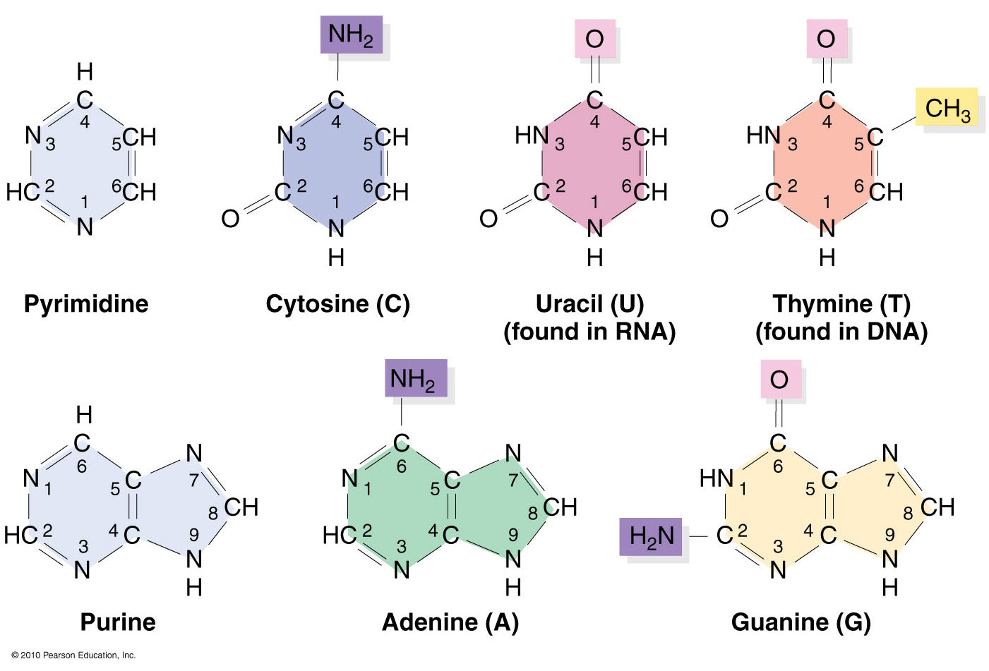
Trained as a chemist, I am aware that the bases are aromatic, heterocyclic compounds (purines and pyrimidines). Moreover, the five standard bases (A, C, G, T, and U) also share a six-membered ring, with atoms named consecutively (N1, C2, N3, C4, C5, C6). This special feature can be employed to identify nts automatically, from PDB atomic coordinates. The ring skeleton is not influenced by protonation states, tautomeric forms, or modifications in base, sugar or phosphate. Early versions of 3DNA (up to v2.0) used only N1, C2, and C6 atoms to identify an nt: an additional N9 as purine, otherwise as pyrimidine. In 3DNA v2.3 and DSSR, the procedure has been refined to take advantage of all available rings atoms. It is thus more robust against distortions and still works even when any of the N1, C2, C6, or N9 atoms are mutated or missing. This blog post provides further technical details on how the method works.

The template used to identify nts is a purine, with nine base ring atoms. Purine is chosen since it contains atoms of the six-membered ring and N7, C8, and N9. Its atomic coordinates in PDB format are shown below. The coordinates are taken from ‘G’ in the standard reference frame ($X3DNA/config/Atomic_G.pdb). Using ‘A’ as reference won’t make any difference since the RMSD between them is only 0.038 Å.

ATOM      1  N9    G A   1      -1.289   4.551   0.000  1.00  0.00           N
ATOM      2  C8    G A   1       0.023   4.962   0.000  1.00  0.00           C
ATOM      3  N7    G A   1       0.870   3.969   0.000  1.00  0.00           N
ATOM      4  C5    G A   1       0.071   2.833   0.000  1.00  0.00           C
ATOM      5  C6    G A   1       0.424   1.460   0.000  1.00  0.00           C
ATOM      6  N1    G A   1      -0.700   0.641   0.000  1.00  0.00           N
ATOM      7  C2    G A   1      -1.999   1.087   0.000  1.00  0.00           C
ATOM      8  N3    G A   1      -2.342   2.364   0.001  1.00  0.00           N
ATOM      9  C4    G A   1      -1.265   3.177   0.000  1.00  0.00           C

The nt-identification process begins with a mapping of at least three atoms in the purine, followed by a least-squares fit between corresponding atoms. For the five standard bases and most modified ones, the RMSD is normally less than 0.12 Å, as seen in the Figure below. Even the unsaturated dihydrouridine in tRNA has an RMSD of less than 0.25 Å: for the yeast phenylalanine tRNA (PDB id: e1ehz), for example, it is 0.205 Å for H2U-16, and 0.226 Å for H2U-17. DSSR uses a cutoff of 0.28 Å, covering essentially all nucleotides in the PDB. As an extreme case, the DA1 residue on chain T of PDB id 4ki4 has only three base atoms: N7, C8, and N9 (i.e., no atoms from the six-membered ring). With an RMSD of only 0.005 Å, DSSR still takes it as an nt, properly assigned as ‘A’.

Molecular dynamics (MD) simulations sometimes produce heavily distorted bases, which is over the default cutoff. Users may change the cutoff to a larger value to accommodate such unusual cases.

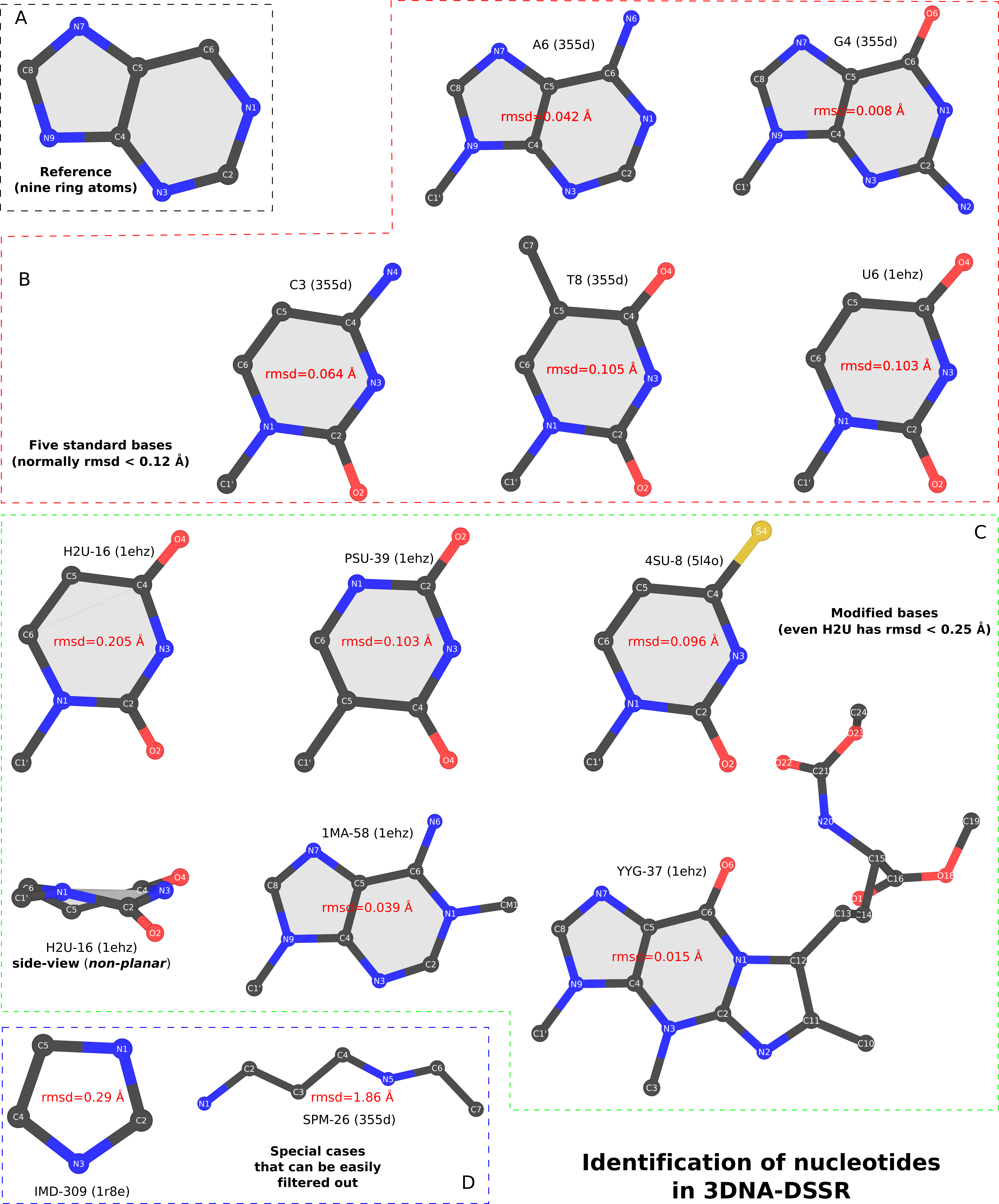
In addition to dihydrouridine, the above Figure also shows pseudouridine (PSU), 1-methyladenosine (1MA), 4-thiouridine (4SU), and the heavily modified YYG in tRNA. They are all easily identified using the same scheme. Since the nt-identification method concentrates on base rings, modifications in sugar or the phosphate group do not pose any problem. For example, in tRNA 1ehz, DSSR also identifies O2’-methylguanosine (OMG) and O2’-methylcytidine (OMC) as modified nts.

Two special cases worth mentioning. The ligand IMD in PDB id 1r8e has a five-membered ring. Its atoms are named similarly to those of an nt, and the fitted RMSD is only 0.29 Å. IMD can be filtered out by its missing of the C6 atom and having an N1—C5 covalent bond. The ligand SPM in PDB id 355d is a linear molecule, and its RMSD (1.86 Å) is clearly far off to be taken as an nt.

Another particular case (of a different kind) is the abasic sites, especially in X-ray crystal structures in the PDB. By definition, abasic sites do not have base atoms available. Thus the described method is not applicable to their characterization as nts. As of v1.7.3-2017dec26, however, DSSR has also incorporated abasic sites into the analysis pipeline, by default. The program checks backbone linkage and residue name for appropriate nt assignment. The abasic sites could constitute part of (internal) loops which would otherwise be broken into segments by DSSR.

Overall, I feel confident to say that 3DNA-DSSR has practically solved the problem of identifying nts from atomic coordinates. The method detailed herein (and outlined in the DSSR paper) is simple and easy to understand/implement. Moreover, it has been extensively tested in real-world applications for well over a decade. I’ve yet to find a single case where it does not work as expected.

Recently, a 3DNA user asked on the Forum about how to perform mutations to 3-methyladenine. The user reported that the procedure described in the FAQ entry How can I mutate cytosine to 5-methylcytosine did not work for the case of 3-methyladenine. This ‘limitation’ is easily understandable: the 3DNA mutate_bases program must have knowledge of the target base, 3-methyladenine, to perform the mutation properly. The program works for the most common 5-methylcytosine mutations since the corresponding 5MC file (Atomic_5MC.pdb, in the standard base-reference frame) is already included within the 3DNA distribution. By supplying a similar file for the target base, mutate_bases runs the same for mutations to 5-methylcytosine (or other bases). This blog post outlines the procedure, using 3-methyladenine as an example.

A ligand name search for 5-methylcytosine on the RCSB PDB led to only two matched entries: 2X6F and 3MAG. The ligand id is 3MA. Since 3MAG has a better resolution (1.8 Å) than 2X6F (3.3 Å), its 3MA ligand was extracted from the corresponding PDB file (3MAG.pdb). The atomic coordinates, excluding those for the two hydrogens, are as below. Note that the 3-methyl carbon atom is named CN3.

HETATM 2960  N9  3MA A 600      16.587  14.258  22.170  1.00 49.87           N
HETATM 2961  C4  3MA A 600      17.123  13.100  21.622  1.00 50.46           C
HETATM 2962  N3  3MA A 600      16.877  11.811  22.009  1.00 50.37           N
HETATM 2963  CN3 3MA A 600      15.983  11.363  23.063  1.00 50.41           C
HETATM 2964  C2  3MA A 600      17.590  10.968  21.241  1.00 50.11           C
HETATM 2965  N1  3MA A 600      18.422  11.217  20.224  1.00 49.27           N
HETATM 2966  C6  3MA A 600      18.627  12.484  19.858  1.00 48.99           C
HETATM 2967  N6  3MA A 600      19.426  12.709  18.829  1.00 46.12           N
HETATM 2968  C5  3MA A 600      17.949  13.503  20.593  1.00 49.89           C
HETATM 2969  N7  3MA A 600      17.929  14.900  20.488  1.00 49.84           N
HETATM 2970  C8  3MA A 600      17.113  15.286  21.434  1.00 49.58           C

After running the 3DNA utility program std_base with options -fit -A, the corresponding atomic coordinates of 3MA are transformed to the standard base reference frame of adenine. The file must be named Atomic_3MA.pdb, and it has the following contents:

HETATM    1  N9  3MA A   1      -1.287   4.521   0.006  1.00 49.87           N
HETATM    2  C4  3MA A   1      -1.262   3.133   0.004  1.00 50.46           C
HETATM    3  N3  3MA A   1      -2.337   2.286  -0.009  1.00 50.37           N
HETATM    4  CN3 3MA A   1      -3.743   2.648  -0.047  1.00 50.41           C
HETATM    5  C2  3MA A   1      -1.905   1.013   0.001  1.00 50.11           C
HETATM    6  N1  3MA A   1      -0.662   0.520   0.004  1.00 49.27           N
HETATM    7  C6  3MA A   1       0.366   1.372  -0.003  1.00 48.99           C
HETATM    8  N6  3MA A   1       1.588   0.867  -0.034  1.00 46.12           N
HETATM    9  C5  3MA A   1       0.068   2.768   0.003  1.00 49.89           C
HETATM   10  N7  3MA A   1       0.875   3.914  -0.003  1.00 49.84           N
HETATM   11  C8  3MA A   1       0.026   4.909  -0.003  1.00 49.58           C

Note that in file Atomic_3MA.pdb, (1) the z-coordinates of the base atoms are close to zeros, (2) the ordering of atoms is as in the original ligand of 3MA shown above.

With Atomic_3MA.pdb in place (in the current working directory, or the $X3DNA/config folder), one can perform 3-methyladenine mutations using mutate_bases. For illustration purpose, let’s generate a B-form DNA with base sequence GACATGATTGCC using the 3DNA fiber program:

fiber -seq=GACATGATTGCC fiber-BDNA.pdb

To mutate A7 to 3MA, one needs to run mutate_bases as following:

mutate_bases "chain=A s=7 m=3MA" fiber-BDNA.pdb fiber-BDNA-A7to3MA.pdb

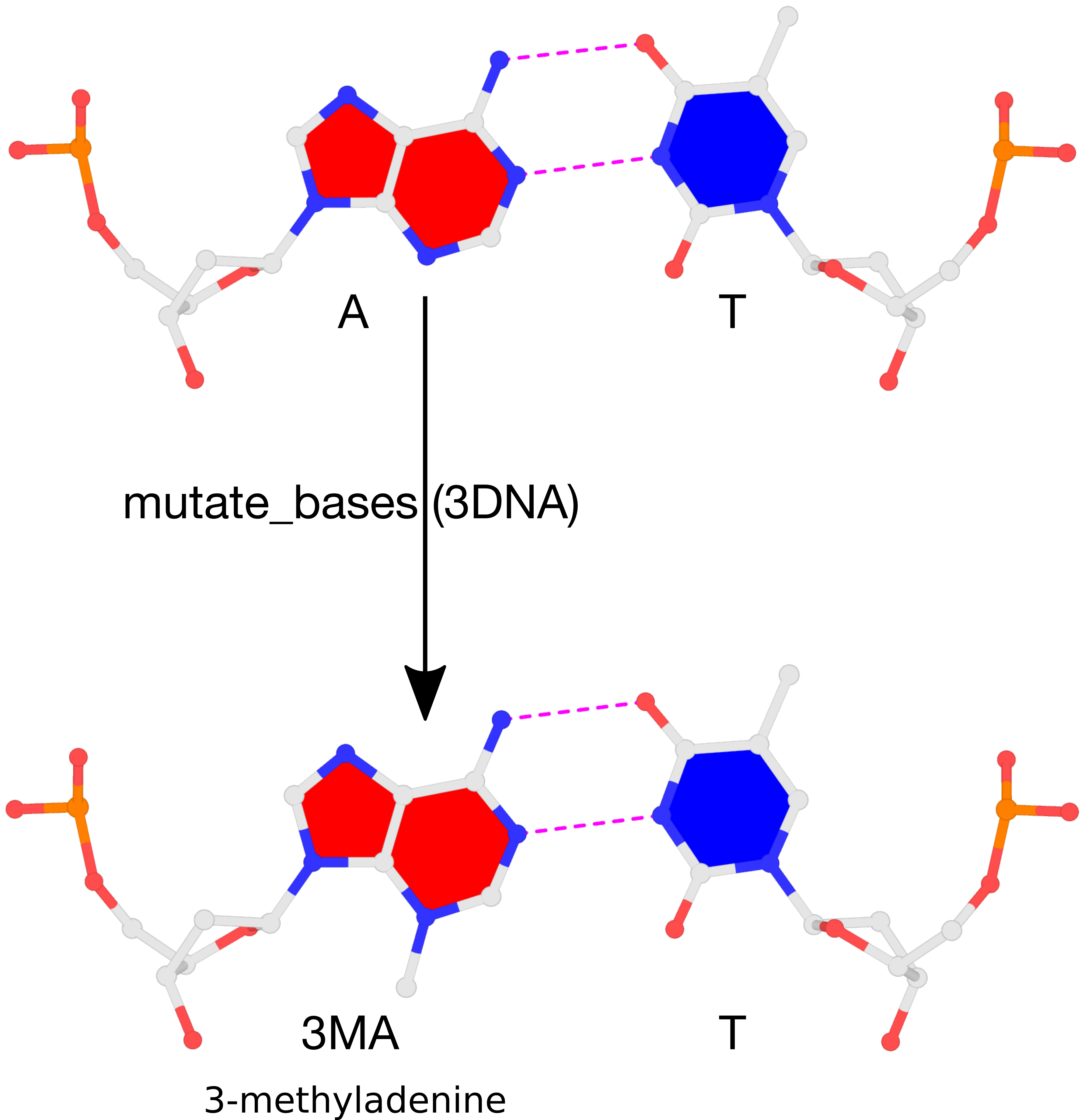
The result of the mutation is shown in the figure below. Note that the backbone has identical geometry as that before the mutation, and the mutated 3MA-T pair has exactly the same parameters (propeller/buckle etc) as the original A-T. These are the two defining features of the 3DNA mutate_bases program.

Please see the thread mutations to 3-methyladenine on the 3DNA Forum to download files fiber-BDNA.pdb and fiber-BDNA-A7to3MA.pdb.

By following DSSR citations, I recently came across the article Interactive Visualization of RNA and DNA Structures by Lindow et al. The paper introduced a DNA/RNA visualization tool that integrates 1D sequence, 2D secondary structure in linear and graph representations, and 3D backbone ribbons and base ladders, all in one package. Notably, the 3D visualization was tailored for DNA/RNA structures and achieved quite impressive results. A nice feature of the 2D graph representation is the handling of multiple chains.

Reading through the main text and the supplementary material, I was surprised to see the so many locations where DSSR was mentioned, especially the following:

Our approach detects all standard and many modified nucleotides as well as the most common base pairs. Further special cases could be easily added. Yet, the system we developed should not be seen as a replacement for well established tools like DSSR. Rather, it shows what can be achieved with modern techniques in terms of both computation and rendering.

Overall, DSSR is an analysis/annotation tool that is supposedly agnostic to visualization programs. It derives a huge number of structural features that are unlikely to be matched elsewhere. I collaborated with Bob Hanson so that Jmol can directly take advantage of what DSSR has to offer, not just for the visualization of (modified) nucleotides and some common base pairs, but also the interactive selection of loops, pseudoknots, coaxial stacks, and various motifs. In particular, the SQL-like selection syntax Bob developed is really flexible and extremely powerful. I collaborated with Thomas Holder so that PyMOL can gain DNA/RNA domain knowledge. The resultant dssr_block PyMOL plugin is quite useful for creating base/base-pair block images with many revealing features, especially for small to medium-sized DNA/RNA structures. It is obvious to me that PyMOL (or any other molecular visualization tool) would benefit greatly from SQL-like selections of DSSR-derived features of nucleic acid structures, just as Jmol does.

In the Lindow et al. paper, some of the references to DSSR are technical in nature. Here, I’d like to respond and clarify each of them. Since DSSR is being actively developed and supported, I always welcome any feedback on the 3DNA Forum. Following and responding to literature represents another way that I strive to make DSSR a better tool to serve the community.

Built on their experience from 3DNA, Lu et al. developed DSSR [27], a very powerful tool to analyze RNA structures that uses Jmol for the 3D visualization. Recently, Hanson and Lu described this integration [10], which is based on a JSON-interface that directly couples DSSR and the 3D visualization of Jmol. This is a great improvement, but still missing is the integration of 2D secondary structure visualizations and brushing & linking techniques to enable simple selection with and exploration of the 3D molecular structure. One contribution of this paper is to show how a full linking between 3D and 2D visualizations can be done and what benefits arise from such a tight coupling (see Sects. 8 and 9).

This is a valid point, and the authors did a good job. Actually, one of the reviewers of our DSSR-Jmol paper brought up this point, and we acknowledged the limitation. While passing DSSR-derived secondary structural features (in DBN or .ct format) to a 2D visualization tool is straightforward, the connection would not be as smooth as we’d like it to be.

For this purpose, other approaches rely on the unique naming and ordering of the atoms [27], for example, N1, C2, N3, C4, C5, C6 etc. We found that this information is not always reliable.

The naming of the purines and pyrimidines follows the IUPAC standard and is a prerequisite of DNA/RNA structures in the PDB. In my experience, I have never found a single case where such information is not reliable. See below for abasic sites in PDB id 3BWP, and 4SU (4-thiouridine) in PDB id 5AFI.

We compared these results with the latest version of DSSR [27]. Our approach is able to correctly detect all regular nucleotides and most of the modified and undefined nucleotides. In the following, we describe the minor differences.

It is not clear what was the “latest” version of DSSR that was actually used in the paper. Note that DSSR has version info as in v1.8.3-2018oct29. I deliberately put the release date along with the version number.

For dataset 4RGE, we detected 3 modified uracil nucleotides that were not labeled as modified by DSSR. These nucleotides have a DNA backbone instead of an RNA one.

DSSR takes A, C, G, T, U as standard nucleotides, even if T is in RNA or U is in DNA. So this result is expected.

Dataset 3BWP contains 7 nucleotides that only consist of the backbone part without bases. While our approach marks these as undefined, in DSSR they are not detected at all.

The 7 nucleotides on 3BWP are abasic sites, i.e., without base atoms (N1, C2, N3, C4, C5, C6 etc), so they do not possess base reference frames. From early on, DSSR had the --abasic option for such cases. As of v1.7.3-2017dec26, DSSR directly incorporated abasic sites into the analysis. So thereafter they are detected by DSSR, by default.

Furthermore, in 5AFI we mark 3 nucleotides as undefined, while these are detected as a modified uracil by DSSR. This is due to the base containing sulfur instead of oxygen, so they possibly are sulfur analogs of uracil.

Presumably, the authors are referring to 4SU, 4-thiouridine, clearly a modified nucleotide occurring in 137 PDB entries (as of 2018oct28). DSSR detects three cases in 5AFI, as shown here: 4SU-u 3 v.4SU8,w.4SU8,y.4SU8

We also compared the results of our base pair detection (Suppl. Tab. 1). We determined all Watson-Crick, Hoogsteen, and Wobble pairs, and the reverse versions of the first two. For most of the datasets, our method returned the same results as DSSR. In particular, both approaches never created contradicting results, which means all common base pairs had identical pair type. In general, our geometrical approach generates slightly more base pairs compared to DSSR. However, when investigating both, the base pairs determined by DSSR but not by our approach and vice versa, we found that most of these pairs are border-line cases, where the decision was made depending on the threshold of the geometrical heuristic. Only in a few cases, the differences were not clear for both approaches, see Suppl. Fig. 3.

In Suppl. Fig. 3,

… However, the hydrogen bonds for classical G-U Wobble pairs seem to be quite unrealistic for the bottom left pair. Either this is a limitation of DSSR or it is some kind of specific Wobble pair with other hydrogen bonds than the depicted ones that our approach does not detect.

I echo the point that border-line cases could cause discrepancies between different methods. However, things can get easily clarified in concrete examples. Unfortunately, the authors did not specify the cases used in their Suppl. Fig. 3. I finally figured out the DSSR-assigned G-U Wobble pair in PDB id 1S72, U2586—G2592. As shown in the figure below, DSSR detects two H-bonds (dashed pink lines), "N3(imino)*N2(amino)[3.05],O4(carbonyl)-N1(imino)[2.77]". Note that one of the H-bonds is between two donors, N3(U) and N2(G), thus the * symbol. The H-bonds are by no means as those in “classical G-U Wobble pairs”. Yet, the pair is clearly Wobble-like, and that’s why it was assigned “Wobble”. To avoid such confusions, I’ve revised DSSR to tighten the criteria of G-U Wobble pair. As of v1.8.3-2018oct29, this pair is called "~Wobble".

Nevertheless, our evaluation (Sect. 8.1) shows that with the proposed approaches in terms of quality we get very similar results to the ones obtained by tools like DSSR. In terms of speed, DSSR needs much longer run times. For example, for 4U4O, DSSR needed ~15 min for the secondary and tertiary structure analysis [27], while our algorithm only needs ~0.2 s (see Tab. 1).

As noted above, DSSR provides far more structural features than just the identifications of nucleotides and several common base pairs. Even for the identified base pairs, DSSR provides many more annotations and structural parameters than just the named pairs picked by the authors. Not surprisingly, DSSR is slower than the dedicated method for a specific purpose.

As of DSSR v1.8.3-2018oct29, I’ve added the --pair-only option that just outputs a complete listing of base-pairing information and then stops. Some sample runs are as below:

x3dna-dssr -i=1ehz.pdb --pair-only
x3dna-dssr -i=1ehz.pdb --pair-only --more
x3dna-dssr -i=1ehz.pdb --pair-only --json
x3dna-dssr -i=1ehz.pdb --pair-only --json | jq '.pairs[] | select(.name=="WC")'
x3dna-dssr -i=1ehz.pdb --pair-only --more --json | jq .
x3dna-dssr -i=4u4o.cif --pair-only -o=4u4o-pairs.txt

Compared to the default settings, DSSR runs ~10 times faster when the --pair-only option is set; 36s vs 5m48s for 4U4O on my MacBook Pro 2017 (2.9 GHz Intel Core i7). Note the timing here is a complete run of the DSSR program (as shown above), from reading the mmCIF file to writing out all the derived features. In my hand, simply reading and parsing the 85MB 4U4O.cif would take ~5s. As a reference, just loading 4U4O.cif into PyMOL takes >6s. I’m thus more than surprised (and remain to be convinced) by the claim that their new algorithm “only needs” ~0.2s “for the secondary and tertiary structure analysis” of 4U4O.

Over the past couple of months, I’ve further enhanced the DSSR-derived structural features for Q-quadruplexes (G4). One was the implementation of the single descriptor of intramolecular canonical G4 structures with three connecting loops recently proposed by Dvorkin et al. The descriptor contains the number of guanines in the G4 stem, the type and relative direction of loops linking G-tracts of the stem, and the groove-widths associated with lateral loops. For example, PDB entry 2GKU (see the DSSR-enabled PyMOL schematic image below, Fig. 1A) has the following DSSR output.

List of 1 G4-stem
  Note: a G4-stem is defined as a G4-helix with backbone connectivity.
        Bulges are also allowed along each of the four strands.
  stem#1[#1] layers=3 INTRA-molecular loops=3 descriptor=3(-P-Lw-Ln) note=hybrid-1(3+1) UUDU anti-parallel
   1  glyco-bond=ss-s groove=-wn- mm(<>,outward)  area=14.24 rise=3.58 twist=16.8  nts=4 GGGG A.DG3,A.DG9,A.DG17,A.DG21
   2  glyco-bond=--s- groove=-wn- pm(>>,forward)  area=13.12 rise=3.71 twist=25.9  nts=4 GGGG A.DG4,A.DG10,A.DG16,A.DG22
   3  glyco-bond=--s- groove=-wn-                                                  nts=4 GGGG A.DG5,A.DG11,A.DG15,A.DG23
    strand#1  U DNA glyco-bond=s-- nts=3 GGG A.DG3,A.DG4,A.DG5
    strand#2  U DNA glyco-bond=s-- nts=3 GGG A.DG9,A.DG10,A.DG11
    strand#3  D DNA glyco-bond=-ss nts=3 GGG A.DG17,A.DG16,A.DG15
    strand#4  U DNA glyco-bond=s-- nts=3 GGG A.DG21,A.DG22,A.DG23
    loop#1 type=propeller strands=[#1,#2] nts=3 TTA A.DT6,A.DT7,A.DA8
    loop#2 type=lateral   strands=[#2,#3] nts=3 TTA A.DT12,A.DT13,A.DA14
    loop#3 type=lateral   strands=[#3,#4] nts=3 TTA A.DT18,A.DT19,A.DA20

The descriptor=3(-P-Lw-Ln) means that the G4 structure has three layers of G-tetrads, connected via three loops: the first is the Propeller loop in anti-clockwise (negative) direction, then the Lateral loop passing a wide groove anti-clockwise, and finally another Lateral loop passing a narrow groove, also anti-clockwise. The DSSR symbols follow those of Dvorkin et al. but with capital letters L, P, and D for lateral, propeller, and diagonal loops instead of lower case letters (l, p, d) to avoid using subscript for groove-width info. So the 2GKU descriptor 3(-P-Lw-Ln) from DSSR corresponds to 3(-p-l_w-l_n) of Dvorkin et al.

The DSSR-enabled, PyMOL-rendered, block image in Fig. 1A makes the three G-tetrad layers (squared green blocks) immediately obvious. Other base identities and stacking interactions also become clear — for example, the A24 (in red) stacks on the top G-tetrad, and T1-A20 pair stacks with the bottom G-tetrad.

Two other PDB entries (2LOD and 2KOW) are illustrated in Fig. 1B and Fig. 1C. They have different topologies than 2GKU (Fig. 1A). DSSR is able to characterize all of them consistently.

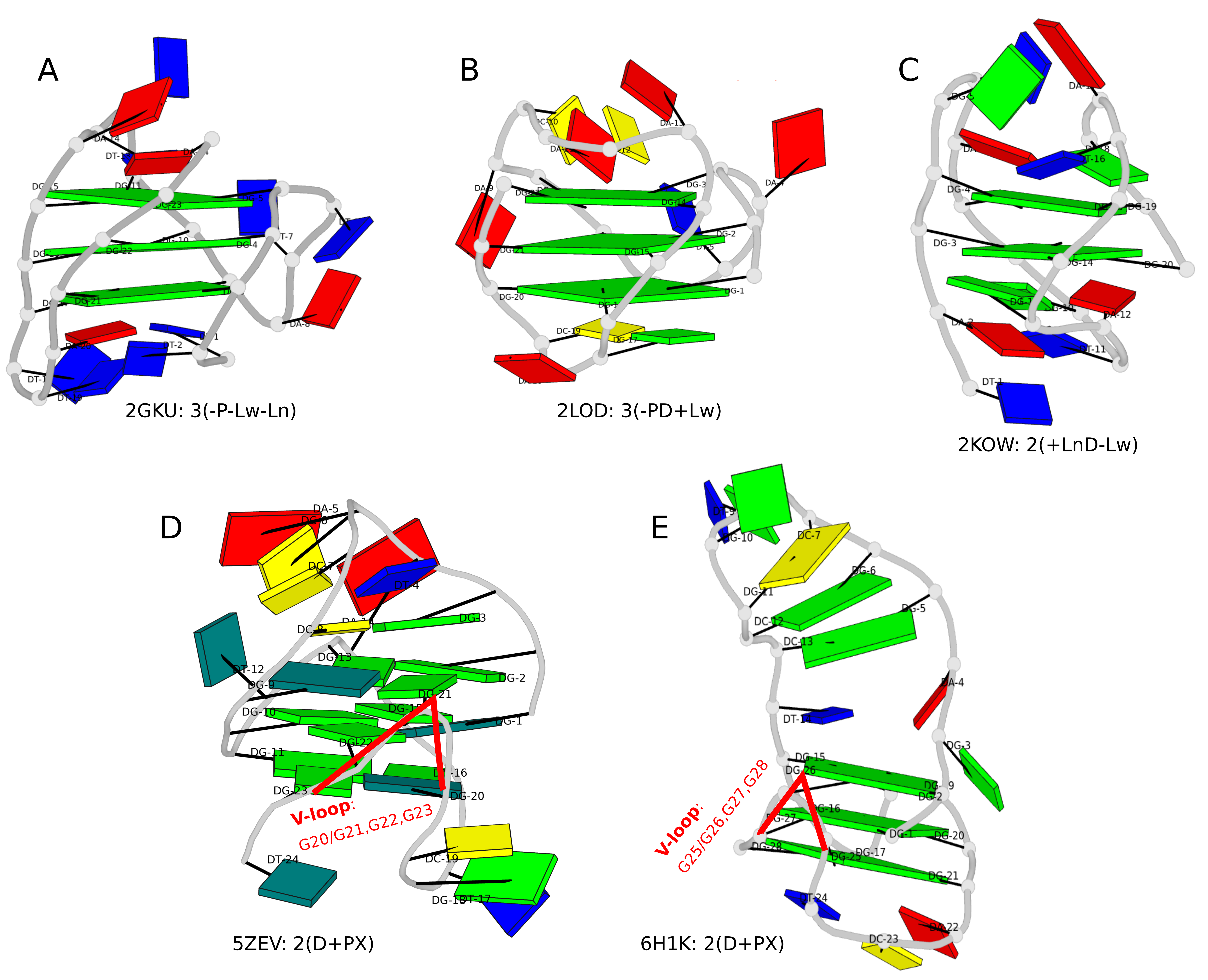
Figure 1. DSSR-enabled, PyMOL-rendered, block images of five G-quadruplexes. A in red, C in yellow, G (and G-tetrad) in green, and T in blue.

Another G4-related new feature in DSSR is the detection of V-shaped loops in noncanonical G4 structures where one of the four G-G columns (strands) that link adjacent G-tetrads is broken. Two of recent PDB examples with V-loops are shown in Fig. 1D (5ZEV) and Fig. 1E (6H1K). An excerpt of DSSR output for the PDB entry 6H1K is shown below.

List of 1 G4-helix
  Note: a G4-helix is defined by stacking interactions of G4-tetrads, regardless
        of backbone connectivity, and may contain more than one G4-stem.
  helix#1[1] stems=[#1] layers=3 INTRA-molecular
   1  glyco-bond=-sss groove=w--n mm(<>,outward)  area=12.76 rise=3.47 twist=18.2  nts=4 GGGG A.DG2,A.DG19,A.DG15,A.DG26
   2  glyco-bond=s--- groove=w--n pm(>>,forward)  area=12.84 rise=3.07 twist=33.4  nts=4 GGGG A.DG1,A.DG20,A.DG16,A.DG27
   3  glyco-bond=s--- groove=w--n                                                  nts=4 GGGG A.DG25,A.DG21,A.DG17,A.DG28
    strand#1 DNA glyco-bond=-ss nts=3 GGG A.DG2,A.DG1,A.DG25
    strand#2 DNA glyco-bond=s-- nts=3 GGG A.DG19,A.DG20,A.DG21
    strand#3 DNA glyco-bond=s-- nts=3 GGG A.DG15,A.DG16,A.DG17
    strand#4 DNA glyco-bond=s-- nts=3 GGG A.DG26,A.DG27,A.DG28

****************************************************************************
List of 1 G4-stem
  Note: a G4-stem is defined as a G4-helix with backbone connectivity.
        Bulges are also allowed along each of the four strands.
  stem#1[#1] layers=2 INTRA-molecular loops=3 descriptor=2(D+PX) note=UD3(1+3) UDDD anti-parallel
   1  glyco-bond=s--- groove=w--n mm(<>,outward)  area=12.76 rise=3.47 twist=18.2  nts=4 GGGG A.DG1,A.DG20,A.DG16,A.DG27
   2  glyco-bond=-sss groove=w--n                                                  nts=4 GGGG A.DG2,A.DG19,A.DG15,A.DG26
    strand#1  U DNA glyco-bond=s- nts=2 GG A.DG1,A.DG2
    strand#2  D DNA glyco-bond=-s nts=2 GG A.DG20,A.DG19
    strand#3  D DNA glyco-bond=-s nts=2 GG A.DG16,A.DG15
    strand#4  D DNA glyco-bond=-s nts=2 GG A.DG27,A.DG26
    loop#1 type=diagonal  strands=[#1,#3] nts=12 GAGGCGTGGCCT A.DG3,A.DA4,A.DG5,A.DG6,A.DC7,A.DG8,A.DT9,A.DG10,A.DG11,A.DC12,A.DC13,A.DT14
    loop#2 type=propeller strands=[#3,#2] nts=2 GC A.DG17,A.DC18
    loop#3 type=diag-prop strands=[#2,#4] nts=5 GACTG A.DG21,A.DA22,A.DC23,A.DT24,A.DG25

****************************************************************************
List of 2 non-stem G4 loops (INCLUDING the two terminal nts)
   1 type=lateral   helix=#1 nts=5 GACTG A.DG21,A.DA22,A.DC23,A.DT24,A.DG25
   2 type=V-shaped  helix=#1 nts=4 GGGG A.DG25,A.DG26,A.DG27,A.DG28

Note that here a new loop type (diag-prop) and topology description symbol (X) are introduced. In developing DSSR in general, and G4-related features in particular, I’ve always tried to follow conventions widely used by the community. Whereas inconsistency exists, I pick up the ones that are in line with other parts of DSSR. For unique DSSR features lacking outside references, I came up my own nomenclature. When DSSR becomes more widely used, it may serve to standardize G4 nomenclatures.

From early on, the --json and --nmr options in DSSR have provided a convenient means to analyze an ensemble of solution NMR structures in the standard PDB/mmCIF format, as those available from the Protein Data Bank (PDB). The usage is very simple, as shown below for the PDB entry 2lod. The parameters for each model can be easily parsed from the output JSON stream.

A practical example of the DSSR JSON/NMR usage for the analysis of RNA backbone torsion angles can be found on the 3DNA Forum.

While not a practitioner of molecular dynamics (MD) simulations, I’ve regularly followed the relevant literature. I know of the popular tools such as MDanalysis, MDTraj, and CPPTRAJ that are dedicated to analyze trajectories of MD simulations. I understand the subtleties MD may have, and I’m also sure of the unique features DSSR has to offer. By design, I made the DSSR interface to MD straightforward, by simply following commonly-used standard data formats: the MODEL/ENDMDL delineated PDB (or the PDBx/mmCIF) format for input, and JSON for output. Overall, I had expected that DSSR would complement the dedicated tools (e.g., MDanalysis, MDTraj, and CPPTRAJ) for MD analysis.

Over the years, DSSR has gradually gained recognition in the MD field. At a meeting, I once heard of a user complaining that DSSR is too slow for the analysis of millions of frames of MD simulations. Yet, without access to a large MD dataset and direct collaborations from a user, the speed issue could not be pursued further. In my experience, I knew DSSR is fast enough for the analysis of NMR ensembles from the PDB. This situation has completely changed recently, after a user reported on the 3DNA Forum on the slowness of DSSR on MD analysis.

Do you have an idea why the backbone parameter for a nucleic acids are so much faster calculated with do_x3dna than with DSSR? Analyzing a trajectory with 100k frames take for a native structure approx. 2 hours with do_x3dna. A native RNA structure with DSSR will take approx. 10 days (10k frames/day). I need to run DSSR, because my system contains an abasic site.

With the above and follow-up information provided, I was able to fix the DSSR algorithm for parsing MD trajectories, among other things. Now DSSR reads a trajectory sequentially frame-by-frame at constant speed. The same 100K frames takes 36 minutes to finish instead of 10 days, which is an increase of 10*24*60/36=400 times. This 100x speedup was later on verified when I tested DSSR on the 1000-structure trajectory the user supplied.

So as of v1.7.8-2018sep01, DSSR is quick enough for real-world applications on MD analysis. In the releases of DSSR afterwards, I’ve further polished the code and added some new features. All things considered, DSSR is bound to become more relevant in the active MD field in the years to come.

By the way, for those who do not like the --nmr option, --md or --ensemble also works. These three alternatives are equivalent to DSSR internally.

As mentioned in the blog post Integrating DSSR into Jmol and PyMOL,
“The small size, zero configuration, extensive features, and robust performance make DSSR ideal to be integrated into other bioinformatics tools.” In addition to the DSSR-Jmol and DSSR-PyMOL integrations which I initiated and got personally involved, other bioinformatics resources are increasingly taking advantage of what DSSR has to offer. Here are a few examples:

• As of Nov. 7, 2017, DSSR has become the only option for base-pairing annotation in the WebSTAR3D web server for RNA 3D structure alignment. In the 2016 WebSTAR3D publication in Bioinformatics, DSSR was the second choice, as shown in the excerpt below:

Before aligning structures, STAR3D preprocesses PDB files with base-pairing annotation using either MC-Annotate (Gendron et al., 2001; Lemieux and Major, 2002) (for PDB inputs) or DSSR (Lu et al., 2015) (for PDB and mmCIF inputs) and pseudo-knot removal using RemovePseudoknots (Smit et al., 2008).

• In the RNApdbee 2.0 web server for RNA secondary structure annotation, DSSR is the default option for identifying base pairs. See also the corresponding publication in Nucleic Acids Research (2018), titled RNApdbee 2.0: multifunctional tool for RNA structure annotation. In contrast, the first version (published in 2014) of RNApdbee put DSSR as the third option, following RNAView and MC-Annotate. See my blog post titled RNA pseudoknot detection and removal with DSSR, and the excerpts from the 2014 (RNApdbee) and 2018 (RNApdbee 2.0) papers:

2014, RNApdbee: In order to facilitate a more comprehensive study, the webserver integrates the functionality of RNAView, MC-Annotate and 3DNA/DSSR, being the most common tools used for automated identification and classification of RNA base pairs.

2018, RNApdbee 2.0: Base pairs can be identified by 3DNA/DSSR (default) (4), RNAView (5), MC-Annotate (3) or newly added FR3D (15).

• The Universe of RNA Structures (URS) web-interface to the URS database (URSDB) makes extensive use of DSSR. For each analyzed structure (including PDB entries), the DSSR text output file (termed “DSSR-file”) is also available. Impressively, the maintainers of URS are quick with DSSR updates. The current version used by the URS website is DSSR v1.7.4-2018jan30.

Forty years after the yeast phenylalanine tRNA structure was solved, modified nucleotides should no longer be an issue for RNA structural analysis, especially for this classic molecule. Automatic processing of modified nucleotides is just one aspect of DSSR’s substantial set of features. Based on my understanding of the field, more structural bioinformatics resources/tools could benefit from DSSR. Simply put, if one’s project is related to 3D DNA or RNA structures, DSSR may be of certain help. It’s just a timing issue that DSSR would benefit a (much) larger community.

Via Google Scholar, I noticed the recent publication in Nucleic Acids Research by Meier et al. titled Structure and hydrodynamics of a DNA G-quadruplex with a cytosine bulge. Reading through the article, I am pleased to see the section “Nucleic acid geometry and visualization” under MATERIALS AND METHODS:

We used the program DSSR (53) of the 3DNA suite (54) to analyse the nucleic acid backbone and the base pair geometry from the 3D structures. We reported the ‘simple’ base-pair parameters for buckle, propeller twist and stagger which are more intuitive for non-canonical base-pairs than the classic base-pair parameters as explained in the program manual and the 3DNA website (http://x3dna.org/highlights/details-on-the-simple-base-pair-parameters, http://x3dna.org/articles/simple-parameters-for-non-Watson-Crick-base-pairs). We wrote an R (55) script that automatically creates a backbone angle plot from the output of the DSSR program. The script can be downloaded from the 3DNA forum at http://x3dna.org. The nucleic acid was visualized in PyMOL and the dssr block plugin (The PyMOL Molecular Graphics Sys- tem, Version 2.0, Schro ̈dinger, LLC, https://pymol.org/). …

This is the first time (I’m aware of) that the ‘simple’ base-pair parameters introduced in 3DNA v2.3 is cited in a peer-reviewed journal article. I’m also glad to know that the blog posts on the 3DNA homepage are read, and even referenced in a publication — which surely will prompt me to write more. This is also the first time that the dssr_block PyMOL plugin is cited. I must say that Figures 1, 5, and 6 from the paper look gorgeous. Among other things, the G-tetrads and the surrounding base identity are immediately obvious using the simple color code: A, red; T, blue, C, yellow, and G, green. See Fig. 1 below.

In the section on “DATA AVAILABILITY”, the authors further noted:

Our R (55) script that automatically creates backbone angle plots from the output of the DSSR program can be downloaded from the 3DNA forum at http://x3dna.org.

I communicated with Markus Meier (the lead author) on the 3DNA Forum, on the thread DSSR: Analyzing NMR structures – overwritten output files. Checking the thread right now, I found that the R script (backbone_torsions_plot-1.0.tar.bz2) has been downloaded 263 times. I appreciate Markus’s effort in contributing the R script with a working example to the DSSR user community. It has always been my hope that more DSSR users would share their scripts and examples via the 3DNA Forum.

As a side note, I met Markus in Los Angles at the 60th Annual Meeting. It was a nice experience chatting with him, and had a lunch together. We’ve kept in touch following the meeting.

When visiting the RCSB PDB website today, I am please to notice that the PDB now contains “10015 Nucleic Acid Containing Structures”. Based on “Macromolecule Type” in “Advanced Search” of the RCSB PDB website, I observed the following information:

• The number of DNA-containing structures is 6,384 (reported in 2,997 papers), and the corresponding number for RNA-containing structures is 3,861 (associated with 2,012 publications).
• There are 4,570 structures containing both DNA and protein (potentially forming DNA-protein complexes), and 2,478 RNA-protein complexes.
• The smallest nucleic-acid-containg structures have only two nucleotides (e.g., 3rec), and largest ones are the ribosomes (and virus particles).
• The earliest released DNA structure from the PDB is 1zna (on March 18, 1981), a Z-DNA tetramer. The earliest RNA structure released is 4tna (on April 12, 1978), a refined structure of the yeast phenylalanine transfer RNA.

This landmark achievement is made possible by the world-wide scientific community through decades of efforts solving DNA/RNA 3D structures via experimental approaches (mainly solution NMR, x-ray crystal, and cryo-EM). These over 10K nucleic acid structures present both challenges and opportunities for the field of structural bioinformatics, especially for intricate RNA molecules. DSSR is an integrated software tool for dissecting the spatial structure of RNA. It is my effort in addressing the challenging issues for the analysis/annotation and visualization of RNA structures.

It is textbook knowledge that the Watson-Crick (WC) pairs are specific, forming only between A and T/U (A–T/U or T/U–A) or G and C (G–C or C–G). Furthermore, an A only forms one WC pair with a T, so is G vs. C. The widely used dot-bracket-notation (DBN) of DNA/RNA secondary structure depends crucially on this feature of specificity and uniqueness, by using matched parentheses to represent WC pairs, such as ((....)) for a GCGA (GNRA-type) tetra-loop of sequence GCGCGAGC.

The reality is more complicated, even for what’s presumably to be a ‘simple’ question of deriving RNA secondary structure from 3D coordinates in PDB. One subtlety is related to the ambiguity of atomic coordinates that renders one base apparently forming two WC pairs with two other complementary bases. As always, the case can be best illustrated with a concrete example. The image shown below is taken from PDB entry 1qp5 where C20 (on chain B) forms two WC pairs, each with G4 and G5 (on chain A) respectively.

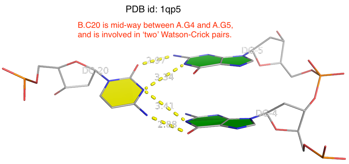
Clearly, taking both as valid WC G–C pairs would make the resultant DBN illegitimate. DSSR resolves such discrepancies by taking structural context into consideration to ensure that one base can only have a WC pair with another base. Here the G5–C20 WC pair is retained whilst the G4–C20 WC is removed.

This issue, one base can form two WC pairs as derived from the PDB, has been noticed for a long while. Two examples from literature are shown below:

• Smit et al. (2008) From knotted to nested RNA structures: A variety of computational methods for pseudoknot removal, RNA, 14(3): 410–416. In the section “Crystal structure data” of “MATERIALS AND METHODS”, the authors wrote:

The crystal structure data files were downloaded from the Research Collaboratory for Structural Bioinformatics (RCSB) Protein Data Bank (Berman et al. 2000). For each crystal structure, the set of canonical base pairs was extracted by selecting all Watson–Crick and standard G-U wobble pairs found by RNAview (Yang et al. 2003). Occasional conflicts in this list, where RNAview annotates two bases, x and y, as a standard base pair and also y and z as another conflicting base pair, were removed manually by visual inspection of the crystal structure in the program PyMOL (http://pymol.sourceforge.net/). The helix-extension data set was created by taking the canonical pairs and adding all additional base–base interactions identified by RNAview (excluding stacked bases and tertiary interactions) for which the direct neighbor was already in the collection. This means each base pair (i,j) was added if both i and j were still unpaired and if either (i + 1, j – 1) or (i –1, j + 1) were already in the set.

• Reinharz et al. (2018) Mining for recurrent long-range interactions in RNA structures reveals embedded hierarchies in network families, Nucleic Acids Research, gky197. In the sections “Data” and “Secondary structure” of “MATERIALS AND METHODS”, the author wrote:

… From these complexes, we retrieved all RNA chains also marked as non-redundant by RNA3DHub. Each chain was annotated by FR3D. Because FR3D cannot analyze modified nucleotides or those with missing atoms, our present method does not include them either. If several models exist for a same chain, the first one only was considered. For the rest of this paper, the base pairs extracted from the FR3D annotations are those defined in the Leontis–Westhof geometric classification (24).

For each chain a secondary structure without pseudoknots was deduced from the annotated interactions, as follows. First all canonical Watson–Crick and wobble base pairs (i.e. A-U, G-C and G-U) were identified. Then, since many structures are naturally pseudoknotted, we used the K2N (25) implementation in the PyCogent (26) Python module to remove pseudoknots. Problems arise when a nucleotide is involved in several Watson–Crick base pairs (which is geometrically not feasible), probably due to an error of the automatic annotation. Those discrepancies were removed with a ad hoc algorithm such that if a nucleotide is involved in several Watson–Crick base pairs, we remove the base pair which belongs to the shortest helix.

By design, DSSR takes care of these ‘little details’, among other handy features (such as handling modified nucleotides and removing pseudoknots). By providing a robust infrastructure and comprehensive framework, DSSR allows users to focus on their research topics. If you have experience with other tools, such as RNAView and FR3D cited above, give DSSR a try: it may fit your needs better.